Excel - Mouse Training London Ltd

Excel Advanced Course

Excel is a vital tool for boosting your efficiency and productivity when you’re dealing with large amounts of data and calculations. This course is a journey through the key topics for Excel power users and majors on Macros and Pivot Tables…

Microsoft Excel Advanced Course

Excel Advanced Course

Excel is a vital tool for boosting your efficiency and productivity when you’re dealing with large amounts of data and calculations. When you understand Excel at a more advanced level, you’ll have the ability to use its more sophisticated tools to streamline your workflow. Our Excel Advanced course is a journey through the key topics for Excel power users and majors on Macros and Pivot Tables.

All our courses are available online with Zoom or Teams. You are welcome to attend our training centre or we can come to you. Call 020 7920 9500 today for further details.

Macros

Create macros to automate your day-to-day Excel work. Save hours of your precious time otherwise wasted on repetitive tasks. Excel has its own command language, VBA (Visual Basic for Applications) We can use VBA to give instructions to get things done.

Specify a series of commands and instructions that you link together to perform tasks automatically. This is a great help with tasks such as saving and copying files from other sources and aggregating data. Get the Excel robot to work for you!

Pivot Tables

You can analyse massive amounts of data with Pivot Tables. On our Excel Advanced course we will examine some of the advanced Pivot Table features. See how to link different tables together with relationships and weave your magic with multi-table reports.

We can use Grouping to aggregate data and visual Slicers to filter our data by different views. Then we shall produce various metrics with Summarize By calculations and use Power Pivot to calculate measures using DAX formulas. We’ll round up the show by doing some serious data crunching with Power Query.

Stand Out. Get Certified!

In addition to our standard courses we also offer certified courses for those taking their MOS exams. MOS (Microsoft Office Specialist) certification is a world-wide recognised qualification that validates your proficiency in using software applications.

The MOS certified course is a 2-day event held at your office, hosted by a MOS certified trainer. You can take the exam online at your office if you wish. Or arrange the exam for whenever it works for you.

The SUMPRODUCT function is one of those hero functions that, once discovered, you wonder how you ever managed without. It does not just do “what it says on the tin”, there’s a lot more to it than that. In particular, it’s one of the most powerful and flexible filter functions in Excel. And so much better than SUMIF or SUMIFS.

It’s easy to calculate someone’s age from their date of birth if you know about Excel’s DATEDIF function, unfortunately it’s easy to miss this function as it is not documented. Excel will not help you fill in the DATEDIF function interval values, you need to see the list here.

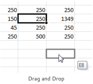
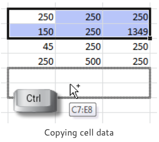
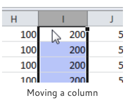
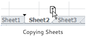
Our Excel double click tricks are some of those little things that make your life so much easier. You probably know most of them already. Or do you? I think that anyone who uses Excel regularly should know them.

Complicated text formulas using either ampersands and the CONCATENATE function are the bane of our life. Not any more! Excel new text functions will really help us nail those text formulas. We’ll be looking at the CONCAT function and the TEXTJOIN function.

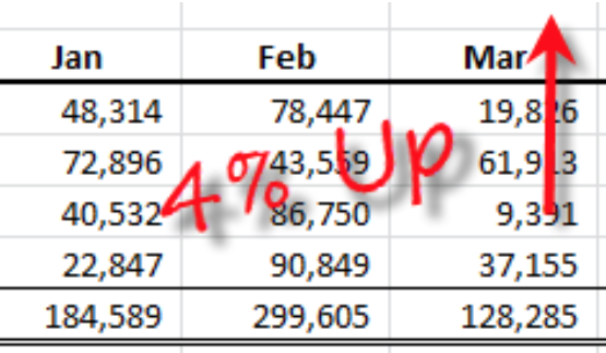
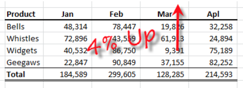
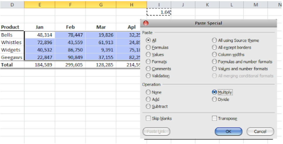
Usually the formulas you need for percentages and differences are quite straightforward: divisions for percentages and a minus sign to take one value from another. But there are pitfalls for the unwary which we shall explore.

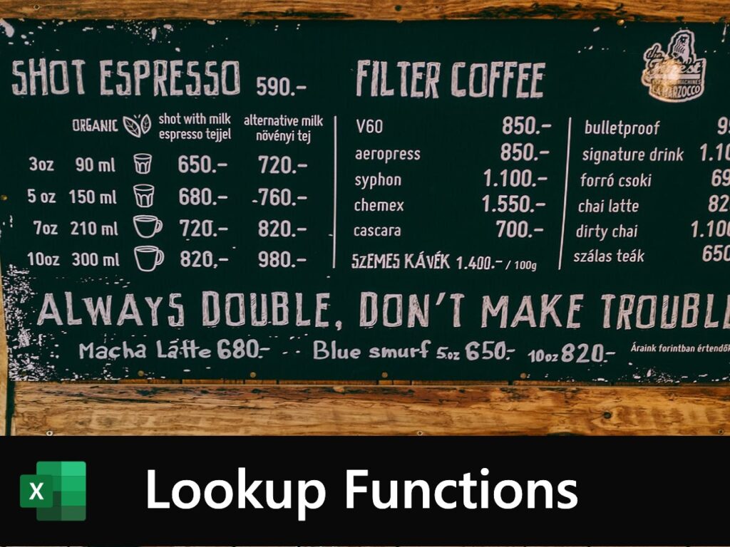
I think the Excel FILTER function does the filter job better than AutoFilter. It’s a live formula and an extraction, you don’t have to filter your data in place. There’s no need for that clunky Advanced Filter…

Essential Excel Functions

Functions are the backbone of most worksheets. But there are around 500 worksheet functions in Excel! Our course covers the most important Excel functions. The ones you will actually use time and time again…

Excel Essential Functions Course

Essential Excel Functions

Functions are the backbone of most worksheets. But there are around 500 worksheet functions in Excel. How can you possibly learn them all? The answer is, of course, you don’t need to learn all of them. But you do need to know Excel’s best ever functions. The ones you will actually use time and time again.

Our one-day training course is devised to give you a broad skill set covering all the primary categories of Excel functions. We will examine how to create filtering calculations using functions like SUMIFS and COUNTIFS. Then concentrate on introducing logical decision-making into our formulas. Make your formulas think for themselves! And, finally, master the use of lookup functions like VLOOKUP.

All our courses are available online with Zoom or Teams. You are welcome to attend our training centre, or we can come to you. Call 020 7920 9500 today for further details.

Filter Functions

Everybody can do a SUM or a COUNT. But, in real life, many of our calculations require some type of filter. Add up all the sales between two dates. Count the number of deals for a specific product. These are examples of filtered calculations. And this where SUMIFS and COUNTIFS are invaluable. Some people would say that you can’t do without them, they are essential functions.

We’ll also deal with the legacy functions, SUMIF and COUNTIF and take a quick look at some of the other handy filtering functions like AGGREGATE and SUMPRODUCT.

Logical Functions

One of the best Excel skills to master is the ability to make your formulas intelligent. Then you’ll start to feel that Excel is working for you. And not the other way round! We shall see how to use functions like IF, IFS and SWITCH to get our formulas to follow a set of simple rules and return different results based on logic.

Mastering logical functions completely changes your formula game. We’ll start by considering the basic if-then-else logic. And then see how to make multiple tests, combine different tests together and how to force out ugly error values.

Lookup Functions

Many people first discover lookup formulas in Excel worksheets that they’ve inherited from their colleagues. Then they realise, with a sense of horror, that these formulas are driving most of the calculations in the worksheet. And they can’t make head nor tail of them!

Don’t let functions like VLOOKUP or MATCH work their mystery on you. Have you ever looked up the price of a Flat White in your local coffee shop? Yes? Then you already understand what VLOOKUP does. Spend a bit of time with us and learn how to use these all-important and essential Excel functions. It’s time well spent.

Microsoft Power BI Courses

The aim of BI (business intelligence) is to make sense of the vast amounts of data that organisations hold. Our Power BI courses help you analyse and visualise your data and thus guide effective business decision making…

Microsoft Power BI Courses

The aim of business intelligence (BI) is to make sense of the vast amounts of data that organisations hold. Our Microsoft Power BI courses help you analyse and visualise your data and thus guide business decision making and management. We provide Power BI courses from beginner to advanced levels. Our courses can be tailored to best suit your requirements.

All our courses are available online with either Zoom or Teams. You are welcome to attend our training centre, or we can come to you. Call 020 7920 9500 today for further details.

Power BI Introduction

Our Microsoft Power BI Introduction training course helps you extract, analyse and comprehend large quantities of data. This will ensure that you can present data in a logical manner and make informed business decisions. Microsoft Power BI (Business Intelligence) is a user-friendly, report-based analytical tool that is transforming the way that businesses read their performance data.

The course starts from first principles and assumes no previous knowledge. You will learn how to link and model your data in Power BI and then create and share visual reports that reveal business insights.

Power BI Advanced

Our two-day Microsoft Power BI Advanced training course is designed for those who are already using Power BI. But they need to explore its features in more depth. It is ideal for business or financial analysts, data scientists and staff.

Learn about the Data Model, its structure and function and how best to share it. Work with more advanced DAX functions to effectively manipulate your business data. See how to use complex Queries for data load. And use bookmarks and buttons to develop an interactive visual interface.

Mastering DAX

Our two-day Microsoft Power BI Mastering DAX (Data Analysis Expressions) training course gives you a deeper understanding of this powerful data manipulation language. Although it’s often described as “simple but difficult”, DAX is a simple language. But it can be quite a challenge to do the calculations you actually need! However, once mastered, effective DAX formulas are the key to getting the most out of your data.

Our course covers how to use DAX to join and generate tables, control table relationships, gain an understanding filters and context and how to use Time Intelligence calculations.

Excel Pivot Tables Course

Pivot Tables are one of Excel’s most powerful features. And one of the easiest to learn! You can summarise and analyse huge amounts of data easily and rapidly. Produce calculations, slicers, dynamic reports and a whole lot more…

Microsoft Excel Pivot Tables Course

Excel Pivot Tables Course

Pivot Tables are one of Excel’s most powerful features. And one of the easiest to learn! You can summarise and analyse huge amounts of data easily and rapidly. Take our one day Pivot Tables course to go from zero to hero. We start from first principles and go on to produce calculations and dynamic reports. You don’t need to know anything about Excel formulas to attend our Pivot Tables course.

All our courses are available online with Zoom or Teams. You are welcome to attend our training centre, or we can come to you. Call 020 7920 9500 today for further details.

Create Great Pivot Table Reports

How are you doing your regular reports? Crunching numbers with calculators and hundreds of bits of paper is no fun. And it’s always against the clock. We’ll show you how to do it with Excel Pivot Table reports. Update your source data, click to refresh your analytical reports and you’re done for another reporting cycle. Easy!

But there’s more to Pivot Table calculations than just a simple SUM or COUNT. We’ll demonstrate the use of calculated fields and items and how to take advantage of the Show Values As options to calculate percentages, comparatives and differences. These are great for showing calculations like variance on previous month or market share etc.

After you’ve crunched your numbers, we’ll show you how to help everyone interpret your data by introducing data graphics like Slicers, Timelines, Charts, Data bars and Traffic lights.

Excel Intermediate Course

Microsoft Excel Intermediate Course

Excel Intermediate Course

Get the best from Excel, it’s one of the most used office applications. But, at the same time, it’s one of the most under-used. Come along on our Excel Intermediate course and open the door to what Excel can do for you. All you’ll need is a basic, working knowledge of Excel worksheets and we’ll take you through the world of Excel formulas and data analysis. If you’ve heard people muttering on about Pivot Tables and VLOOKUPs then this is the course for you!

Our Excel Intermediate course is available online with either Zoom or Teams. You are welcome to attend our London training centre, or we can come to you. Call 020 7920 9500 today for further details.

Essential Formulas

Some people come out in a rash just thinking about Excel formulas. Don’t despair, they’re not that difficult and you don’t need to be an expert. However, you do need some essential knowledge and be familiar with some of the functions. On our Excel Intermediate course, we’ll show you all you need. See how to add-up numbers quickly and accurately. Then link worksheets together using formulas and see how to easily calculate differences and percentages. And deal with those tricky situations where some formulas need to have dollar signs entered.

Functions are the backbone of Excel formulas. You can come along on our whistle-stop tour of the most useful Excel functions. We’ll use Excel date functions to work out the working days between two dates. Then see how to calculate someone’s age from their date of birth. Filtering functions like SUMIFS and COUNTIFS should be known by everyone. Logical functions like IF and IFS help your formulas think for themselves and lookup functions like VLOOKUP and XLOOKUP are essential Excel skills.

Data Analysis

Excel is brilliant for data analysis. And it’s so easy! We’ll start by seeing how to transform and clean-up raw data using Flash Fill and text formulas. Then we shall summarise and analyse the results with a Pivot Table report.

Our colleagues need to understand and interpret the results of our analysis. This is where Excel data graphics really shine. We’ll see how Charts, Sparklines, Data Bars, Traffic Lights and Heatmaps make the data more natural for the human mind to comprehend.

Keep Your Excel Skills Up to Date

There’s been quite a few changes to Excel in recent years and they’re easily missed. Our New Functions course covers functions like XLOOKUP, FILTER and many more. Number crunchers should check out our Power Query course…

Keep your Microsoft Excel Skills Up to Date

Update Your Excel Skills

Excel is one of the most used office applications. At the same time, it’s one of the most complex. And with so many different disciplines to master: formulas, charts, macros, pivot tables and so on, it’s easy to miss something crucial. Or something that’s new! Try taking a look at our courses and keep your Excel skills up to date.

Our Excel 365 New Functions course showcases all the new functions that have been appearing in Excel in recent years and demonstrates what you can achieve with the new Dynamic Array formulas.

Our other featured course is Excel Power Query. Power Query has been available in Excel for the past few years but falls into the “I never realised that it was there!” category. It’s a crying shame that so many people have not been taking advantage of Power Query to crunch their worksheet data. We hope that our course will give you a few ideas. And save you hours of work.

All our courses are available online with Zoom or Teams. Or you are welcome to attend our training centre. Or we can come to you.

Excel 365 New Functions

Our Excel 365 New Functions training course gets you bang up to date with the quiet revolution that’s been going on with Excel formulas recently. Most of us have relied on familiar functions like VLOOKUP and nested IFs for years. That’s now had a major overhaul. Update your Excel skills.

Don’t worry, all the original functions are still supported. But new functions like IFS, LET and XLOOKUP will completely change your formula game. Making them more powerful and efficient.

Excel’s new calculation engine introduces a new type of function, Dynamic Arrays. We can do calculations that we’d never even thought about doing before. Because now you can easily work with multiple values at the same time in a formula. Dynamic Arrays solve some very tricky problems in Excel formulas and fundamentally change the way our worksheets are designed and constructed.

Excel 365 Power Query

Our Excel Power Query training course is ideal for you if you have to spend time every month cleaning and transforming data. And that’s before you can even begin to analyse it and incorporate it into your reports. Stop the eternal copy and paste, automate your workflow!

We show you how to import data from many different sources. Then combine, transform and reshape your data as required for your Pivot Tables and other Excel reports. You set up your query once and then reuse it with a simple refresh. It’s like a macro, but without the code! For years so many of us have had to write VBA macros to manipulate our data, now you can update your Excel skills by discovering the power of Power Query. Power Query is built into Excel.

Excel Converting USA Dates to UK Dates

Converting USA Dates to UK Dates

Excel Converting USA Dates to UK Dates. Usually Excel date values don’t cause any problems, you just type them in with either slash or dash separators. Don’t bother about the year value unless your date is for a year other than the current year. Excel automatically enters the current calendar year if you just give day and month values.

Country Setting for Dates

However, you will have a problem with the date evaluation if the country setting on your system has not been set correctly. Excel was written in the USA and uses their Month-Day-Year date convention. You will have to change the country setting if you want to use the UK convention of Day-Month-Year.

The United States Declaration of Independence is clearly dated “July 4 1776” so there’s very little chance of their changing the date convention. You can’t argue with the Founding Fathers.

The system country setting issue is easily resolved. Just Google Change the regional settings if you’re not sure how to do it. The real date problem arises when you have to share documents with your friends and colleagues from across the pond. Your opposite number in New York emails you data that was quite sensible when it was entered. When you open the document the dates go haywire.

Reversing the Date Evaluation

You can Google formulas that will reverse the date evaluation for you but they are awkward to implement if you have to do this sort of thing regularly. In this article we are going to create a Date Converter that reverses the day and month values of any date directly in the cell without having to use formulas.

The converter uses an Excel macro which is triggered when you click a shortcut button on your Quick Access Toolbar (QAT). You click the button, select the range of cells containing your dates and you’re done!

Converting UK Dates to USA Dates

It also works the other way round. So, if someone from the London office sends you a spreadsheet and the dates are entered in good-old-King-George Day-Month order you just select your cells and click your shortcut. The date evaluation is whizzed around into nice, sensible Month-Day dates.

Making the Date Converter macro

There’s ten steps to go through here but don’t let that put you off as they are very simple and the entire process will only take a few minutes. If you’re not familiar with the term “macro” then allow me to explain. Macro is short for macro-instruction and is a sequence of instructions written in Excel’s scripting language, VBA (Visual Basic for Applications)

Step 1. Recording a macro

The first step is to record a macro into your Personal Macro Workbook. This is a hidden workbook that is opened automatically whenever Excel starts up, any macros saved in this workbook will always be available for you to use.

Go to the Macros control which is found on the extreme right-hand side of the View tab on the Excel ribbon. Click the bottom section of the control and choose Record Macro from the menu.

Step 2. Using the Personal Macro Workbook

There is very little to do here other than to make sure that you record a macro in the right place.

When the dialog is displayed, change the Store macro in setting to Personal Macro Workbook. It’s available in the drop down list. Don’t bother with anything else. Click OK to start the recorder.

Whatever you do now gets recorded but there’s no need to do anything. Just turn off the recorder and this step is completed. Click Stop Recording in the menu on the Macros control.

Step 3. Finding the recorded macro

We have now created a module (Excel’s storage area for macros) in the Personal Macro Workbook. The next step is to find this module, remove the recording and replace it with the instructions that will do the date conversion work for us.

This is done in the Visual Basic Editor. Press ALT+F11 to open the editor and then see if you can spot a window in the top left-hand corner which looks like this illustration. That’s the Project Explorer window. If you can’t see it, press Ctrl+R.

Look in the listing under PERSONAL.XLSB, you may have to click the plus sign nodes to open up the listing. If you’ve never used the Personal Macro Workbook before you will need Module1. If there are a set of modules visible then you need the last one. Double-click the module and you will display the code of your recording in the window on the right-hand side of the screen.

Step 4. Copying and Pasting the code for the macro

Your recorded macro code will look something like this illustration. Don’t worry if it doesn’t as we are going to delete it and substitute our own code. Select all your code from the word Sub to the words End Sub and press the DELETE key.

Then copy and paste the code from the section below to replace the original.

This is the code for the date converter macro:

Public Sub DateConverter()

Dim rngCells As Range

Dim rngCell As Range

Dim strMsg As String

Dim intDay As Integer

Dim intMonth As Integer

Dim intYear As Integer

Dim DateValue As Date

On Error Resume Next

strMsg = “Select the cells to convert:” & _

vbCr & vbCr & “Reverses Month and Day date evaluation,” _

& vbCr & “i.e. MM-DD becomes DD-MM if possible.”

‘Receive the input.

Set rngCells = Application.InputBox(strMsg, “Date Converter”, , , , , , 8)

‘Test for no input received.

If Not IsObject(rngCells) Or rngCells Is Nothing Then

GoTo Exit_DateConverter

End If

‘Date Conversion Loop.

For Each rngCell In rngCells

If IsDate(rngCell) Then

intDay = Day(rngCell)

intMonth = Month(rngCell)

intYear = Year(rngCell)

DateValue = intMonth & “/” & intDay & “/” & intYear

rngCell.Value = DateValue

End If

Exit_DateConverter:

End Sub

Make sure that you copy and paste everything, starting with the word Public and ending with words End Sub. When you’ve pasted the code you will see that some of the words will turn a blue colour and some green. That’s exactly what they should do.

Step 5. Saving the macro

Now save the workbook. PERSONAL.XLSB is a hidden workbook so save it now as it’s tricky to do it later. Choose File, Save from the main menu.

The macro is completed and we now get back to Excel by pressing ALT+F11 again. Or you can close the Visual Basic Editor window.

Step 6. Creating a shortcut for the macro

In the next few steps we shall create an attractive, easy to use shortcut for the macro.

The most obvious place to have this is on your Quick Access Toolbar. Point to the QAT (top left-hand corner of the Excel window), right-click and choose Customize Quick Access Toolbar from the shortcut menu.

Step 7. Customizing the Quick Access Toolbar

Excel’s Options dialog will display and the Quick Access Toolbar section is activated.

Working from the top left-hand corner of the section, click the Choose commands from drop-down list.

Then click Macros in the list.

Step 8. Assigning the macro to the QAT

Your macro will be displayed in the list on the left-hand side. Select the macro and click the Add command button.

Your macro now appears in the right-hand list which shows you all the shortcuts available on your Quick Access Toolbar.

The next step is cosmetic and will make your shortcut button more visually attractive. Click OK now if you want to skip this final step.

Step 9. Modify the macro button

Click the Modify command button if you want to change the icon displayed for your macro and change the descriptive ‘Screen-Tip’ that pops up whenever you point at the icon.

There’s an array of different icon images to choose from. Enter some text into the Display Name box to set the Screen-Tip text.

You don’t have to enter “Date Converter”, you can enter anything you like. Click OK to close the dialog and OK again to close the main Options dialog.

Step 10. Test the macro

Everything’s done but you always want to test it to make sure. Enter a few dates into your worksheet. Click the Date Converter button on your Quick Access Toolbar. Select the date cells when the input box appears. Click OK and all the dates get switched around.

Using the Date Converter

This is the input box that appears when the shortcut is clicked. Your current cell selection in the worksheet is not detected. Instead, you point out of the box and select a range of cells or a column on your worksheet. All the dates in the selection have their month and day values reversed. Anything that is not a date is ignored.

Congratulations on a successful result and I hope that you enjoyed the Excel converting USA dates to UK dates article.

Related Courses

Microsoft Excel Advanced – Link

Microsoft Excel VBA Introduction – Link

Excel Calculations without Formulas

Excel Calculations Without Formulas

Excel Calculations without Formulas. If you use Excel on a regular basis then you probably know all about formulas and functions but it’s too easy to get into a mental rut and neglect some of Excel’s simpler operations. Here’s a typical example, my worksheet contains the Sales Forecast figures for the next few months and I’ve just been told that I now have to increase all the figures by 4%.

So what do you do? Copy and Paste all the numbers to another worksheet, write a formula to multiply everything by 1.04 then Copy and Paste Special as Values to fix the numbers and finally, copy all the new numbers back to the original worksheet. Well, you could but….

Paste Special Operations

Instead of removing the numbers to another worksheet and doing formulas you can manipulate the cell values in place. Type the multiplier value of 1.04 into an empty cell (any cell will do) and then copy it. Now that you have your value on the Clipboard you can apply it to the numbers.

Select your numbers and then choose Paste Special and in the Operation section click the Multiply option button. Click the OK button and all your numbers are uplifted by 4%. You don’t need the 1.04 multiplier in the cell any more and you can delete it whenever convenient.

Halving numbers, doubling numbers, converting negatives to positives (multiply by minus 1), adding one set of numbers to another or subtracting. These tasks can all be effected without writing a single formula. The Paste Special command is usually available in the right-click shortcut menu or the Edit menu or the Paste control on the Home tab for newer Excel versions.

Finding the Numbers in a worksheet

When you have numbers in a worksheet that you need to select and you don’t want to have to do the selection yourself try using Go To Special.

For example, in the previous example I wanted to select the numbers on a worksheet so that I could multiply them. I did not want to select the cells containing formulas, just the cells with normal numbers or, in Excel speak, the numeric constants.

Choose Go To Special and then click the controls to specify what class of worksheet data you want to have selected. In this case, the Constants option button and the Numbers check box. Click the OK button and Excel selects those values wherever they are on the active worksheet.

Should you select a range before choosing Go To Special then the cell selection is confined to the currently selected range.

So, where is Go To Special? It depends on the version of Excel that you are using, if you have one of the older versions with the drop down menus then you should choose Edit, GoTo and then click the Special command button. In newer Excel versions with the ribbon, go to the Find & Select control on the extreme right hand side of the Home tab, click the control and it’s in the drop down menu.

Related Courses

Microsoft Excel Introduction – Link

Microsoft Excel Intermediate – Link

Excel CTRL Key Tricks

The Excel CTRL key tricks. That dull, grey-beige looking key that lives an unassuming, lonely life on the edge of your keyboard actually leads an exciting double life in Excel. Now, this is not going to be a life changing experience for you but it may bring a touch of fun into otherwise unexciting everyday tasks. Read on.

Copying and Moving Worksheet Cells

Cut and Paste is most peoples’s favourite method of moving data from one cell to another. A simpler alternative is Drag and Drop; point to any of the cell’s borders, wait for the arrow pointer to display and then drag your data to another cell.

If you want to drag your selection onto another worksheet, drag down to the sheet tabs and then hold down the ALT key to switch over to the other worksheet.

To change your move into a copy (Copy and Paste), hold down the CTRL key as you drag. You should see that a plus sign is displayed next to the arrow pointer. Keep your CTRL key held down until you have released the mouse button.

Cell drag and drop is usually enabled. Should you find that the arrow pointer does not display then you need to turn it on. The settings is in Excel Options (File tab), Advanced section, Editing options: Enable fill handle and cell drag-and-drop.

Copying and Moving Columns and Rows

Drag and Drop works in exactly the same way for moving or copying entire columns or rows. Just click the column letter or row number first to select it and then point to the edge of the selection. Drag to move or CTRL+Drag to copy.

Copying and Moving Worksheets

You’ve already figured it out; the drag and drop method is equally effective for copying and moving entire worksheets. Point to the sheet tab and click, the document icon will display. Now drag to the left or right hand side to move the worksheet into a new position in the workbook.

To make a copy of an entire worksheet, point to the sheet tab and click. When the document icon displays, hold down the CTRL key and you will see a plus sign displayed on the icon. Now, drag the sheet to the left or right hand side to create a copy. Try doing that with Copy and Paste.

On some keyboards you need to hold down the CTRL first before clicking the sheet tab.

If your worksheets are in different workbooks then you can still drag and drop your worksheets but you need to have both of the workbooks visible first. Arrange the documents on the screen by clicking the View tab, then go to the Window group and click Arrange All, Tiled. Drag to move a worksheet, CTRL+Drag to copy.

Drag and Drop with the Shift Key

Don’t forget the SHIFT key. When you drag and drop one cell onto another you usually overwrite the data in the destination cell or range of cells.

But when you hold down the SHIFT key as you drag then you insert cells into the destination range without overwriting data.

Watch the I-beam as you drag, the vertical I-beam means Shift cells right and the horizontal I-beam means Shift cells down.

In the illustrations we took the 450 cell value over to the right and dragged it into the E5 cell position and the rest of the cell range moved down to accommodate the data insertion.

Filling Data with the Fill handle

The Fill handle is that little black cross-shaped mouse pointer that appears at the lower right corner of the active cell. Not unreasonably, it is popularly known as the “little black cross”. When you drag the Fill handle down or across you fill the data from the active cell across or down: formulas are copied, numbers are copied as constants and text stored in an Custom list, such as days of the week, triggers the list sequence.

When you hold down the CTRL key as you drag you will see a plus sign displayed on the black cross and this reverses the normal behaviour of the fill. For example, if you drag a cell containing the value of 1 then the number 1 will remain constant but if you hold down the CTRL key then you will generate the sequence of values: 1,2,3,4 etc.

Normal text is copied as a constant but Custom list text is entered in the order of the custom list. Custom lists can be very handy; for example you type “March” into a cell then you drag to enter the other months of the year.

But this can be irritating if you wish the month name to remain constant. This is where you hold down the CTRL key to reverse the usual action. Type in “March” and then CTRL+Drag to copy “March” into the cells below.

Excel Custom lists can be viewed, edited and set up in Options (File tab), Advanced section, scroll down to General and click the Edit Custom Lists control.

Repeating Patterns with the Fill handle

Sequences of numbers may be generated by creating a seed pattern in a few cells and then selecting this seed pattern and dragging to extend the sequence. For example a plus 10 sequence is seeded by typing 10 and 20 into consecutive cells, then you select the two cells and drag to generate the sequence 10,20,30,40,50 etc.

Repetitions of the seed pattern are obtained by holding down the CTRL key as you drag. The sequence of values is then repeated; 10,20,10,20,10,20 etc.

Making Multiple Selections

A multiple selection of cells is where you select one range of cells and then you hold down the CTRL key and keep it held down as you continue to add to your initial selection and create a collection.

If you make a mistake then there’s nothing to be done other than to click a cell to clear your current selection and start over again.

This sort of selection is so useful for cell formatting as you can apply your formats to the entire selection in one fell swoop instead of having to format each range individually and invaluable where you want to plot cell ranges which are not immediately adjacent to each other on an Excel chart.

The same method of selection is easily applied to entire columns or rows by clicking the first column letter or row number, then you hold down the CTRL key and click on the others.

With multiple rows selected you can apply actions such as deletion to all the selected rows or with multiple columns selected, as in the illustration, you can change the width of alternate columns in your worksheet. The more you use collections the more ideas you will have. Not all actions can be applied to a multiple selection but it is always worth experimenting.

Now we’ve got the general idea. In the illustration below we coloured alternate sheet tabs red in one go by holding down the CTRL key and clicking on the relevant sheet tabs. Right-click any selected tab to access the Tab Color command.

And the Shift Key again…

The other method of selection that is useful to know is Block selection which uses the SHIFT key. This is the selection of a continuous range of cells effected not by dragging, as is usual, but by clicking. You click the first cell of your selection, hold down the SHIFT key and then click the last cell. It’s Click, Shift, Click.

This feels very awkward if you never tried it before as you can not stop yourself from dragging but if you practice the technique on small ranges of cells then you will rapidly master it. And then you can apply in so many different situations: selecting huge ranges of cells, ranges of sheet tabs etc.

Now you’re an expert in the dark art of Excel cell selection you will find that you can use these selection techniques on other Excel objects and in other Microsoft Office applications.

Extend Mode

A final word on multiple selection, using your keyboard. The CTRL key with a normal mouse is the easiest thing in the world, you hold the key down with your left hand and select with your right hand. But left-handers don’t always have such an easy time of it and some touch pads can make you wish that you had a third hand. This is where you need Extend Mode with the keyboard.

Press function key F8 to open extend mode and then select your first cell range either using your mouse or by using your keyboard: hold down the SHIFT key and extend the selection by pressing your arrow keys.

Now, lock your current selection by pressing SHIFT+F8 and then move on to make your next selection. This is best done by pressing the arrow keys to exit the current selection and then pressing SHIFT and arrow keys again to make the next selection. Press SHIFT+F8 again to lock this selection and continue in this way until the selection is complete.

I can assure you that this is a lot easier to do than it is to read about it.

Related Courses

Microsoft Excel Introduction – Link

Microsoft Excel Intermediate – Link

Excel Drop Down Lists

There are three different types of Excel drop down lists available:

“Pick from” lists which are generated automatically.
Data Validation lists which are very easy to do.
Combo box and List box controls which require a bit more work.

Pick from lists

As you type a list of data into a column in your worksheet you are automatically prompted with previously entered list elements that match your typed characters. In the illustration, I have typed in an “f” and the cell is filled-in with “fred” as this entry is already in the list.

To accept the prompted text, press ENTER or press the Down Arrow key. To decline the suggestion, keep typing.

To generate the list entries without your having to do any initial typing, you can use the shortcut key combination ALT + Down Arrow to display the list elements and then, if you’re a keyboard fan, press the Down Arrow key again to go down through the list and then ENTER to accept the entry.

If you can’t be bothered with all this good old-fashioned shortcut keys business then just right-click in the cell and choose Pick from Drop-down list in the shortcut menu.

Data Validation lists

These lists are used where you want to restrict the entry made in a cell to only those items available in a drop-down list. The list of valid entries can be typed in or you can refer to a range of cells which contains your valid entries. The range of valid entries can be entered into a different worksheet in the same workbook.

Data Validation lists are ideal not only where you need to make sure that people make the right entry but also for data entry generally as it is so easy to choose from a drop-down list. To create the validation list, select the cell or range of cells where you want the list to be displayed and then click the Data Validation control on the Data tab (look for Data Validation in the Data menu if you are using an older version of Excel)

In the Settings tab, choose List from the Allow drop-down list and then type in a comma-separated list of your valid entries into the Source box. In this case, the list items are Yes, No and Maybe. Click the OK button and you’re done. The list is available when you click on one of the cells where the validation has been applied and data entry into the cell is restricted to only those items in the list.

Click the Error Alert tab if you want to change the standard “the value you entered is not valid” error message for invalid entries. You may prefer something a little more personal.

Using a range of cells to provide the source

A range of cells is preferable for your data validation where you either have a long list or you want to be able to change the list regularly.

You can set the Source data validation as either a horizontal or vertical range of cells or an entire column or row. Either type in the range reference or (far easier) select the range or click the column letter or row number.

When you click the column letter remember that any heading at the top of your list on the worksheet will be included as the first item in your validation list. But if you add to the list on the worksheet then these additional items will automatically appear in the validation list. So there are advantages and disadvantages to selecting the whole column.

If you specify a range of cells then then you don’t have the headings issue to deal with but if you then add to the list on the worksheet then you will also have to remember to reset the Source data range to include your additions.

Displaying the drop-down list in alphabetical order

The drop-down list is linked to the values in the worksheet cells, so sort the list in the cells in alphabetical order if you wish to show the drop-down list in the same order. But you can’t have the drop-down list in a different order.

Dependant Data Validation lists

Sometimes you need the choice that you have made in one list to control the list shown in another cell; one of your validation lists is dependant on the other.

In the illustration there are two columns, the first column shows the class of date required, “Month” or “Day”. This is entered from a simple comma separated validation list which is typed in. The second column needs to show either a list of months if “Month” is entered in the corresponding cell in the first column or a list of days if “Day” is entered.

There are two ranges of cells in the worksheet named as Month and Day respectively which are going to be the alternative source ranges for the second column (see the next section if you are not sure how to Name a range) When you set the source data range for the second column enter the following formula: =INDIRECT(A2)

Where A2 is the first cell in the first column where you have your “Day” or “Month” entry. Of course, you should change this cell reference to suit your own worksheet. The INDIRECT function is well named as it makes the reference indirect, i.e. not A2 but the range reference entered in A2. In other words, if it’s “Day” then show the Day list, if it’s “Month” then show the Month list. You’re not restricted to just having a choice between two alternative lists, with this method you can have the choice of as many different lists as you like.

If this does not seem to work for you then try checking the following points:

Did you select the area for the dependant range before applying the Data Validation? In the example above it would have been the second column. It’s very easy to apply validation to a single cell when you intended to set it for a range.
Check the spelling of the range names (in this case “Day” and “Month”) in the first list. They must be spelled correctly and you have to remember them as you type them in as comma separated values.
Did you remember to name the ranges?

Naming a Range

If you’re not sure how to name a range of cells then I would recommend using the Name Box, which is that area on the extreme left-hand side of the formula bar where you normally see your active cell reference. It’s not the only way of naming a range but most people find it to be the easiest way.

Type in the name (in this example it is “Months”) and then press the ENTER key to register the name correctly. Please don’t click out of the box after typing the name, press ENTER. Sorry for being boring but that’s where it’s so easy to go wrong. Click the drop-down arrow to check that the name is available.

Combo box and List box controls

These are interactive graphics which are drawn on top of the worksheet cells and are then linked to certain key worksheet cells. They are commonly employed as a user-friendly graphical device to make user-unfriendly processes involving formulas much easier to control.

In the above example, there is a combo box control containing a list of months. When a month is selected from the list the heading in the worksheet report is updated (“Sales Report for …”) and the relevant monthly numbers are extracted from another worksheet where the full twelve month’s Forecast Sales figures are entered.

All this is done by using Excel formulas but you don’t need to know anything about the formulas to use the worksheet. You just choose a month from the drop down list. Combo box and List box controls are quite easy to do, the hard bit is doing all the formulas.

Form controls

There are two sets of graphical controls available in Excel, Form controls and ActiveX controls. They both do much the same job but in rather different ways so it doesn’t matter which set you use.

Form controls were designed and built for Excel, ActiveX controls are more general controls used in many different applications. Form controls are simple and robust whereas ActiveX controls are more sophisticated and the process of using them takes far longer. It’s a judgement call. I shall be using Form controls in this example and deal with ActiveX in a future article.

Finding the Form controls

This is the first job. Form controls are not openly available, you need to display the Developer tab on your Excel ribbon. Click the File tab and then click Options. Click Customize Ribbon and then click the Developer check box in the Main Tabs list on the right-hand side. Click OK. Form controls are in the Insert control on the Controls group of the Developer tab.

Click the Insert control, the Form Controls are the top group. The Combo Box (1) control is the second one in from the left. The List box (2) control is second in from the right. Both controls behave the same; the Combo box is a drop-down list, the List box is an open list.

Creating the Combo Box

You need to go through a few steps to get the Combo box working. Firstly, create some cell ranges where you are going to store the data that you want to have displayed in the drop-down list and a cell to link the Combo box to. When you format your Combo box these ranges are going to be your Input range and your Cell link.

Personally, I would always put these data ranges on a separate worksheet so that I can then hide it. In the example I shall be using Named Ranges, as they are so easy to work with, rather than normal cell references but this is just personal preference. Use Named Ranges or the standard A1-style cell references as you prefer, they both work fine.

In the illustration, I have a list of my twelve months (shortened for clarity) these are the grey cells and are named MonthList. The pink cell is going to be the cell link and is named MonthPick and the green cell is MonthName, where I am going to enter a formula which will calculate the current month. Now it’s time to create the Combo box, there’s three steps:

Draw and format the Combo box
Set the Input Range and Cell Link
Test the Combo box and the enter the formulas

Draw the Combo box. Click the Combo box control and then drag to draw a horizontal rectangular shape. You can resize it later if it’s not quite right. Right-click the control to display its shortcut menu. Try to right-click when your mouse pointer is pointing to the middle of the control as there are different shortcut menus available, you want the one that contains Format Control.
Format the Combo box. In the Format Control dialog enter the Input Range (in this example MonthList) and the Cell link (MonthPick) Click OK.
Test the Combo box. Click a worksheet cell to take the focus away from the Combo box. It’s now active. Click the drop-down arrow and choose an item from the list. You should see that a value is returned into your link cell. It’s an index value, it’s not the text from the list. If you choose “March” from the list then the index is the value of 3 because it’s the third item in the list.

That’s the Combo box control completed and now it’s time to enter our formulas in the worksheet to make everything happen.

Entering the formulas

When you choose a month from the list you want to trigger the following processes in your formulas:

Update the month name definition. This formula goes in the cell named MonthName so that we can use the name in our formulas wherever we need the selected month declared.
Update the report heading with the name of the month.
Update the report by showing the relevant data for the selected month.

1. Formula in the MonthName cell

Use the index value MonthPick to return the relevant item from the MonthList list using Excel’s INDEX function. The formula is:

=INDEX(MonthList,MonthPick)

2. Update the report heading with the name of the month

The named range MonthName updates to show the currently selected month so we concatenate it’s value with the static text “Sales Report for …”. This formula is entered on the worksheet where we have our report. The formula is:

=”Sales Report for “&MonthName

3. Update the Sales Forecast figures to show the currently selected month

There’s various ways of doing this but the most obvious way is to use the index value MonthPick in a Lookup formula to return the current month’s figures from the range containing all the year’s Sales Forecast figures.

In the illustration above, the grey cells are named SalesForecast. This range is on a different worksheet but that’s not a problem when we use a named range. When the selected month from the Combo box is “March” then the value of MonthPick is 3. The corresponding “March” figures are in the 4th column of the SalesForecast range so if we add the value of 1 to MonthPick then we calculate the correct column index value for our lookup formula. The formula is:

=VLOOKUP(B5, SalesForecast, MonthPick+1, FALSE)

Where B5 is the cell reference of the first Product in the main report (it contains the text “Product 1”), SalesForecast is the lookup range, MonthPick+1 the column index value and FALSE because it is an Exact Match VLOOKUP based on matching the product name in the main report to the products listed in the first column of the lookup range.

Related Courses

Microsoft Excel Intermediate – Link

Microsoft Excel Advanced – Link

Microsoft Excel Advanced Course

Excel Advanced Course

Macros

Pivot Tables

Stand Out. Get Certified!

Related Posts

Excel Essential Functions Course

Essential Excel Functions

Filter Functions

Logical Functions

Lookup Functions

Related Posts

Microsoft Power BI Courses

Microsoft Power BI Courses

Power BI Introduction

Power BI Advanced

Mastering DAX

Related Posts

Microsoft Excel Pivot Tables Course

Excel Pivot Tables Course

Create Great Pivot Table Reports

Related Posts

Microsoft Excel Intermediate Course

Excel Intermediate Course

Essential Formulas

Data Analysis

Related Posts

Keep your Microsoft Excel Skills Up to Date

Update Your Excel Skills

Excel 365 New Functions

Excel 365 Power Query

Related Posts

Excel Converting USA Dates to UK Dates

Table of Contents

Converting USA Dates to UK Dates

Country Setting for Dates

Reversing the Date Evaluation

Converting UK Dates to USA Dates

Making the Date Converter macro

Step 1. Recording a macro

Step 2. Using the Personal Macro Workbook

Step 3. Finding the recorded macro

Step 4. Copying and Pasting the code for the macro

Step 5. Saving the macro

Step 6. Creating a shortcut for the macro

Step 7. Customizing the Quick Access Toolbar

Step 8. Assigning the macro to the QAT

Step 9. Modify the macro button

Step 10. Test the macro

Using the Date Converter

Related Courses

Excel Calculations Without Formulas

Table of Contents

Paste Special Operations

Finding the Numbers in a worksheet

Related Courses

Excel CTRL Key Tricks

Table of Contents

Copying and Moving Worksheet Cells

Copying and Moving Columns and Rows

Copying and Moving Worksheets

Drag and Drop with the Shift Key

Filling Data with the Fill handle

Repeating Patterns with the Fill handle

Making Multiple Selections

And the Shift Key again…

Extend Mode

Related Courses

Excel Drop Down Lists

Table of Contents

Pick from lists

Data Validation lists

Using a range of cells to provide the source

Displaying the drop-down list in alphabetical order

Dependant Data Validation lists

Naming a Range

Combo box and List box controls

Form controls

Finding the Form controls

Creating the Combo Box