Excel AutoSum Revisited

You just can’t get away from AutoSum. If I had a pound for every time I’ve clicked AutoSum to add up a column of numbers I would probably be sitting on a tropical island somewhere still clicking it to add up all my vast wealth. It’s one of the first things you learn about in Excel and, of course, everybody knows it inside out.

Column and Row Totals

Here’s a really easy way of calculating column and row totals without having to do all that infernal copying. The first job is to select all the cells containing your numbers and extend the selection to the empty cells where you want the totals.

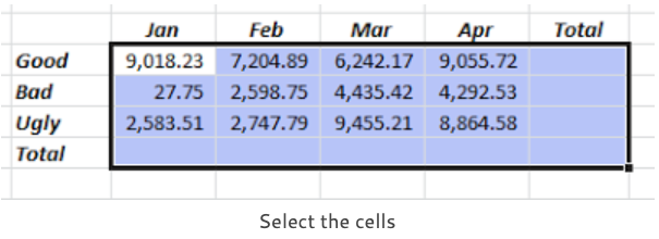
Then you click AutoSum and you’re done! It really is that easy. If you only want the column totals then just select the cells with the numbers and the totals are returned into the row below.

Here’s all the column and row totals done in two simple steps. And they are done perfectly as the range references in the SUMs are implied by the selection. They hardly need to be checked.

If you prefer to do the whole thing with your keyboard then hold down the SHIFT key and extend the cell selection by pressing the arrow keys. Then use the shortcut key combination ALT= to generate the SUM formulas.

Grand Totals

But it’s not just one table is it, you’ve got loads of them and some serious number crunching to do. You can extend the select-and-click-AutoSum method to do grand totals as well. But, be careful, this method only really works if every line item in your worksheet is drawn into a subtotal.

Firstly, calculate all of your individual subtotals and then make a selection of all of the cells containing your numbers and the cells containing your subtotals.

Now, click AutoSum and all the cells containing your subtotal SUMs are detected and the Grand Total is calculated correctly without any risk of double-counting.

Here’s the resulting formulas displayed in the cells and you clearly see the formulas containing the original range references for the subtotal SUMs.

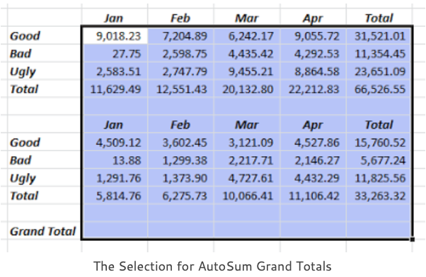
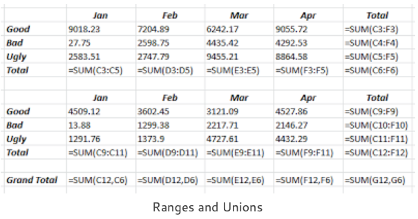
All the grand total SUMs generated by AutoSum are Unions, showing each subtotal reference separated by commas. Number-crunching never has been much fun but this certainly better than having to construct Grand Totals from plus signs and cell references.

Our SUM formulas usually contain Range References, using a colon separator. For example, C3:C5 means “from C3 to C5”. Union references use commas. For example, C12, C16 means C12 and C16.

Checking your Formulas

As some of us know from bitter experience it is very embarrassing when a simple mistake in your formulas messes up all your careful calculations. So, it’s always a good policy to check that you’ve got your formulas right but it’s a bit painful to view them individually in the formula bar.

You can display the formulas directly in the cells by clicking the Show Formulas control. It’s in the Formula Auditing group of the Formulas tab. Click once to show the formulas and click again to show the results.

If you have a really old version of Excel then you have to search in the Tools, Options dialog for this option which is not much fun and I recommend that you use the shortcut key combination CTRL ` (that’s usually the key under the ESC key on the top right of your keyboard) Press the keys once to display the formulas and again to show the returned results.

Related Courses

Microsoft Excel Intermediate – Link

Microsoft Excel Advanced – Link