Blog - Mouse Training London Ltd

Word Doing it with Styles

Word Styles

Word, doing it with styles. Do you spend ages formatting the text in your Word documents? If that’s a “yes” then the bad news is that you’ve possibly been spending far more time than you need to. The good news is that you can save a huge amount of time doing your formatting if you get into the habit of using Styles. And there are many other benefits, as we shall see…

Applying Styles

All of the text in a Word document is in the Normal style. The format of the Normal style is defined by the document template, usually the Normal template. If you are not used to using styles then you don’t bother with any of this. You just select your text and change its format. That’s fine as far as it goes but you’re not really getting the best out of Word unless you use styles. The fundamental way to format text in Word is to apply a style, particularly where you have headings and subheadings.

Heading Styles

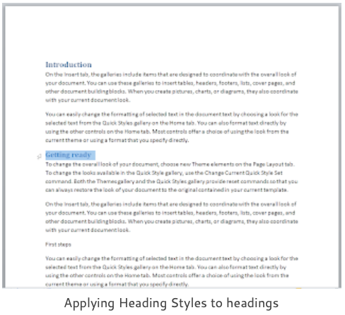
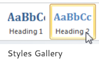
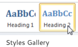
To apply a style to your headings and subheadings, select them one by one and apply a Heading Style from the Styles Gallery on the Home tab.

Use the built-in Heading styles that you can see in the gallery: Heading 1, Heading 2, Heading 3 etc.

Don’t worry if you don’t like the look of your headings because you can always change them later. Not by changing their format but instead by changing the definition of the heading style. Once a style has been applied you can change it as many times as you like. And in as many different ways as you like.

To change the appearance of all the body text in your document you modify the Normal style. To change all the main headings, you modify the Heading 1 style etc.

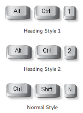
The built-in heading styles go from Heading 1 to Heading 9 and you can apply them using shortcut keys. The shortcut keys only go from ALT+CTRL+1 for Heading1 to ALT+CTRL+3 for Heading3. Three levels of headings is usually enough for most documents. The key combination CTRL+SHIFT+N to apply Normal style is a good one to know for when you apply a heading style by mistake.

Word formats everything with styles. You can usually see where they have been applied just by looking at the text. There is a very handy document view, Draft View. Many people prefer the Draft View to the usual Print Layout View as it lets them see exactly which style has been applied to each paragraph.

When your styles have been applied you can modify them as you like. If you prefer the appearance of your styles to the standard template styles then you can change the default. Then your text looks exactly as you want it to on every new document.

Draft View

Word’s Draft View is designed to show only the text formatting and gives a simplified view of the layout of the page. You can type and edit swiftly in this view. Most people don’t bother with it and much prefer the standard Print Layout view. The draft view is invaluable when you need to see exactly what’s going on with your styles.

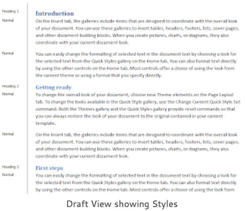
Usually you can tell by the appearance of a heading that you have styled it.

What you can’t see are your mistakes, such as where you have managed to apply Heading 1 to some white space. Or maybe you’re just a control freak. Do you always have that urge within you where to need to know exactly what’s happening?

To show the view, click the Draft control on the View tab. Your style definitions are not normally shown in this view. You must change a Word Options setting in order to see them properly. When you have changed the property, the styles are shown on the left hand side. You only ever have to do this once.

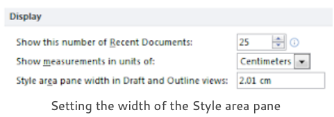
Set the width of the Style Area Pane

To set the width of the style area pane, click the File tab, Options, Advanced, Display section and locate the Style area pane width in Draft and Outline views: control. Enter a suitable width, around an inch or 2cm is about right.

Modify your Styles

Very few people find the appearance of the built-in styles suitable for their purposes. All you have to do is Modify your built-in styles to get exactly the font, paragraph and other formatting that you want.

Then you can either change the Word defaults so that you never have to do this again. Or create a single Style Set which you can apply to the whole document in one step.

The whole point about styles is that you never actually do any formatting apart from applying a style. When you change the properties of the style then everything with that style in your document gets changed.

Changing the Normal Style

For example, many people like to change the font being used in a document and do this by selecting all the text and then choosing a different font from the font control.

This works fine but paragraphs have over a hundred different properties and if you then wanted to say, change the line spacing as well, you would have to go through the whole selection routine again. And then you change your mind…

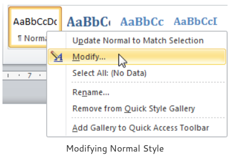
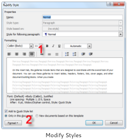
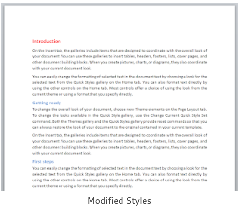
The alternative and much easier method is to modify the Normal style. Right-click Normal style in the Styles gallery on the Home Tab. In the illustration we changed all the body text in the document with a few clicks in the Modify Style dialog. Change the font style, size and justification using the controls in the Formatting section (1). Then click the Format button (2) to change the paragraph formatting.

Changing the Heading Styles

Repeat the same process to change the appearance of the heading styles. Don’t forget to click on the text where the heading style has been applied first before you modify it. There’s nothing more annoying than changing a paragraph of body text to Heading 1.

You don’t like the look of the twenty or so headings in your document? Click on one of them and modify the heading style. The change goes through the entire document.

Or would you prefer to do twenty selections and around another forty formatting clicks to change all your headings? No contest.

Benefits of using Styles

Applying styles ensures speed, consistency and stability in your document. Speed, one change to a style ripples through the document irrespective of how long it is. Consistency, everything formatted with a style complies with the style. Were my main headings 18pt or 16pt? If you have to do them individually then you’re bound to get some of them wrong. Stability, you can not delete an in-built style. Under certain circumstances it may reset to its default values but it’s always there.

Saving your Styles

After all that hard work modifying your styles you will not want to repeat it. If you know exactly what you want for all new documents then change the default. This changes the standard Word document template on which all new documents are based. It does not change documents that you have already created.

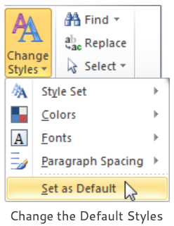
Click the Change Styles control on the Home tab and choose Set as Default. Alternatively, you can create a Style Set which consists of a collection of style definitions. Then you can have your own collection of Style Sets which you can apply to different types of document.

Create a Style Set

To create a Style Set, click the Change Styles control, choose Style Set and Save as Quick Style Set from the fly-out menu. Enter a suitable name for your style set and Word saves it as a template. Whenever you want to apply the style set, click anywhere in your document and choose the style set from the list displayed.

Cleaning Up Existing Documents

Usually it’s best to do all of your document formatting with styles but that’s not always possible. Sometimes you have a document that you’ve already started formatting or, more likely, you inherit documents from other people. These documents can be an amazing mixture of all sorts of styles and fonts. What you want is a nice, clean document that you can format from scratch.

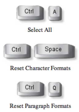
Select all of the text in the document by pressing CTRL+A and then press CTRL+Space to remove any character formatting (colours, fonts, bold, italic etc.) Finally, press CTRL+Q to reset any paragraph formatting (alignment, space after etc.)

All the paragraphs revert to their default values. Any heading styles used will remain in place but all the additional formatting is removed.

Using your Styles

Identifying your body text and your different levels of headings gives your document a structure. A structure that Word can use for a variety of useful tasks. The following sections are a brief guide to how Word can use your styles. And make it well worth the effort of applying them.

Navigation Pane

If you’re sick of having to scroll up and down through long documents then you will really appreciate Word’s Navigation Pane which opens on the left hand side of the Word window. It gives you a bird’s-eye view of the headings in your document.

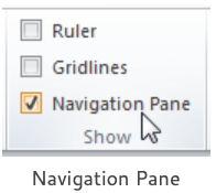
To show the Navigation pane, either click the relevant checkbox in the Show group of the View tab or press the shortcut key CTRL+F. Click the leftmost icon tab in the pane to browse through your headings.

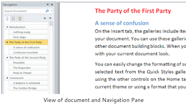
Using the Navigation Pane

Click one of the headings in the Navigation pane and you move to that place in the document. This alone would make me happy but you can also reorganise your work in this pane by dragging and dropping the headings.

The two other tabs in the pane show either thumbnails of each page or Search.

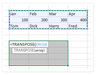
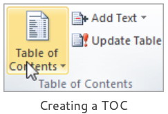
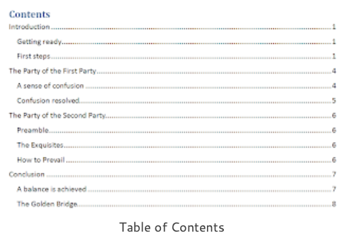
A Table of Contents (informally known as a “TOC”) is a summary list of the contents of your document with numbered page references. It is typically included after the title page. You can easily generate a TOC based on your heading styles, click in your document where you want to insert the TOC and then click the Table of Contents control on the References tab and choose one of the Built-in tables.

The Table of Contents is a snapshot of the current state of the document. When you update your document don’t forget to update your TOC to reflect the changes you have made. Click anywhere in the TOC, the entire table is selected and shaded (it’s a Word field) then click the Update Table control or press F9.

TOC styles control the appearance of the TOC and you can modify them if you don’t like the look of your TOC. They are available in the Styles Window, to see this window either click the dialog launcher at the lower right of the Styles group of the Home tab or press the keys ALT+CTRL+SHIFT+S. When you can see your TOC styles, right click or click the drop-down arrow on the style. Choose Modify from the shortcut menu.

Hyperlinks and Cross-references

Hyperlinks are those underlined and coloured words that you see in web pages. When you click the link you jump to another page or location. You can insert them into Word documents to jump to a web page, an email address or, more commonly, a Place in This Document.

Creating a Hyperlink

Word Hyperlinks create a convenient navigation structure for anyone reading your document. To create one, click the Hyperlink control in the Links group on the Insert tab. Click Place in This Document and you will see all your headings listed on the right hand side. If you don’t want to link to a heading then you must create a Bookmark first and then link to it. Your Bookmarks will be listed under the headings.

To create a Bookmark select some text in your document and click the Bookmark control. Enter a name for the Bookmark and click the Add button. Bookmarks are place holders in the document, you can’t actually see them unless you choose Options, Advanced, Show Document Content.

Creating a Cross-reference

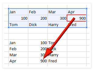
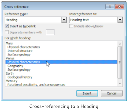
Word can create Cross-references to your headings or bookmarks which can be updated as the document changes. For example, we have some heading text, “Geography” to which we have applied the Heading 2 style and we wish to create a cross-reference that reads like this, “See Geography on page 4“.

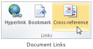
Click where you want the cross-reference, type in the word “See” followed by a space. Then click the Cross-reference control.

Choose Heading from the Reference type list and Heading text from the Insert reference to list. Click the Insert button. That gives you the “Geography” bit and it will update should you subsequently change the text of the heading. Finish off the cross-reference by typing ” on page ” and then repeat the process but this time choose Page number from the Insert reference to list.

Updating your References

Whenever you want to update your cross-references and make sure that their information is up to date, select the entire document by pressing CTRL+A and then press function key F9 to update everything.

Paragraph Numbering

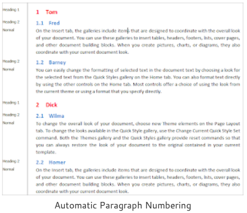
Word heading styles are ideal when you want sequential paragraph numbering in a hierarchy that goes something like this: 1, 1.1, 1.2, 1.3, 2, 2.1, 2.2 etc. What you need is a List Style which will group existing heading styles and relate them to each other. Fortunately, Word contains a library of built-in List Styles which are easily applied and you can also create your own to suit.

Using a List Style

Create your document and apply the various heading styles to your headings as usual. You don’t actually do any numbering yourself, instead you let the heading styles and the List style apply the numbering for you.

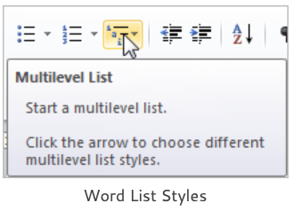
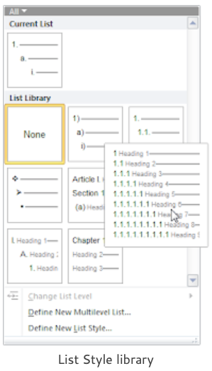
Select all the text in your document by pressing CTRL+A and then click the Multilevel List control in the Paragraph group on the Home tab. Or just click at the start of the document, there’s really no need to select any text once your styles are applied. Browse the List Library and select one of the Lists which are clearly based on the heading styles and Word will number all your paragraphs automatically.

If you can’t find a List Style that works for you then you will have to create your own. This is not the easiest of tasks but it’s the only way if you want something special. Click Define New List Style in the Multilevel List menu.

In the Define New List Style dialog, enter a name for the list then click the Format button and choose Numbering. Click the More button and then link each list level to your heading styles and set the number style and formatting.

Outline View

Word’s Outline View is often neglected. This is a shame as it is the best tool for the job when you are having to manage long documents such as reports, proposals, contracts etc. These documents usually have several sections and require extensive editing and reorganisation before the final version is produced.

Create your document as usual and apply heading styles to the headings. Click the Outline control on the View tab to turn on the Outline view.

In this view you see a condensed version of the full document showing the normal body text paragraphs and the headings shown at their various levels. Heading 1 style corresponds to Level 1, Heading 2 style corresponds to Level 2 etc.

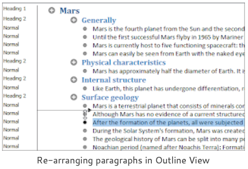
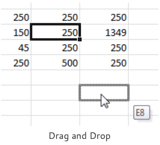
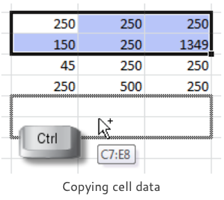
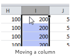
It is now so easy to reorganise your document, all you have to do is drag and drop a heading to move the heading and all its associated subheadings and body text. There’s absolutely no need for all that selection and cutting and pasting work that so many people inflict upon themselves.

When you have set up automatic paragraph numbering you will see that all the numbering updates to comply with the new structure. You can use shortcut keys if you don’t want to drag and drop the headings. Click a heading and then press ALT+SHIFT+Up Arrow or ALT+SHIFT+Down Arrow to move that section up or down in the document.

Creating a PDF file

Word’s built-in heading styles are easily interpreted as PDF bookmarks. One of the most useful additions that you can make to most PDF’s is to create bookmarks for navigation. PDF bookmarks are the clickable objects shown on the left of the Adobe Acrobat window that you use to expand and collapse the headings and show the different levels. Much the same idea as Word’s Navigation pane.

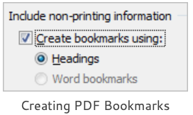
Creating bookmarks manually is a very painful task. But there is no need to bother with that as you can set the built-in headings in your Word file as PDF bookmarks when you save the document as a PDF file. Click the Options button in the Publish as PDF or XPS dialog and check the checkbox Create bookmarks using and the option button Headings.

Doing it with Styles Conclusion

That’s the end of the Word styles propaganda. As we’ve seen, Word formats everything with styles. But it’s not just document formatting where styles can help us get our work done efficiently, there’s quite a few other things a well. If you’ve been using Word for a bit and you’ve not yet tried using styles, give them a go and see if they work for you.

Related Courses

Microsoft Word Intermediate – Link

Microsoft Word Advanced – Link

Excel Converting USA Dates to UK Dates

Converting USA Dates to UK Dates

Excel Converting USA Dates to UK Dates. Usually Excel date values don’t cause any problems, you just type them in with either slash or dash separators. Don’t bother about the year value unless your date is for a year other than the current year. Excel automatically enters the current calendar year if you just give day and month values.

Country Setting for Dates

However, you will have a problem with the date evaluation if the country setting on your system has not been set correctly. Excel was written in the USA and uses their Month-Day-Year date convention. You will have to change the country setting if you want to use the UK convention of Day-Month-Year.

The United States Declaration of Independence is clearly dated “July 4 1776” so there’s very little chance of their changing the date convention. You can’t argue with the Founding Fathers.

The system country setting issue is easily resolved. Just Google Change the regional settings if you’re not sure how to do it. The real date problem arises when you have to share documents with your friends and colleagues from across the pond. Your opposite number in New York emails you data that was quite sensible when it was entered. When you open the document the dates go haywire.

Reversing the Date Evaluation

You can Google formulas that will reverse the date evaluation for you but they are awkward to implement if you have to do this sort of thing regularly. In this article we are going to create a Date Converter that reverses the day and month values of any date directly in the cell without having to use formulas.

The converter uses an Excel macro which is triggered when you click a shortcut button on your Quick Access Toolbar (QAT). You click the button, select the range of cells containing your dates and you’re done!

Converting UK Dates to USA Dates

It also works the other way round. So, if someone from the London office sends you a spreadsheet and the dates are entered in good-old-King-George Day-Month order you just select your cells and click your shortcut. The date evaluation is whizzed around into nice, sensible Month-Day dates.

Making the Date Converter macro

There’s ten steps to go through here but don’t let that put you off as they are very simple and the entire process will only take a few minutes. If you’re not familiar with the term “macro” then allow me to explain. Macro is short for macro-instruction and is a sequence of instructions written in Excel’s scripting language, VBA (Visual Basic for Applications)

Step 1. Recording a macro

The first step is to record a macro into your Personal Macro Workbook. This is a hidden workbook that is opened automatically whenever Excel starts up, any macros saved in this workbook will always be available for you to use.

Go to the Macros control which is found on the extreme right-hand side of the View tab on the Excel ribbon. Click the bottom section of the control and choose Record Macro from the menu.

Step 2. Using the Personal Macro Workbook

There is very little to do here other than to make sure that you record a macro in the right place.

When the dialog is displayed, change the Store macro in setting to Personal Macro Workbook. It’s available in the drop down list. Don’t bother with anything else. Click OK to start the recorder.

Whatever you do now gets recorded but there’s no need to do anything. Just turn off the recorder and this step is completed. Click Stop Recording in the menu on the Macros control.

Step 3. Finding the recorded macro

We have now created a module (Excel’s storage area for macros) in the Personal Macro Workbook. The next step is to find this module, remove the recording and replace it with the instructions that will do the date conversion work for us.

This is done in the Visual Basic Editor. Press ALT+F11 to open the editor and then see if you can spot a window in the top left-hand corner which looks like this illustration. That’s the Project Explorer window. If you can’t see it, press Ctrl+R.

Look in the listing under PERSONAL.XLSB, you may have to click the plus sign nodes to open up the listing. If you’ve never used the Personal Macro Workbook before you will need Module1. If there are a set of modules visible then you need the last one. Double-click the module and you will display the code of your recording in the window on the right-hand side of the screen.

Step 4. Copying and Pasting the code for the macro

Your recorded macro code will look something like this illustration. Don’t worry if it doesn’t as we are going to delete it and substitute our own code. Select all your code from the word Sub to the words End Sub and press the DELETE key.

Then copy and paste the code from the section below to replace the original.

This is the code for the date converter macro:

Public Sub DateConverter()

Dim rngCells As Range

Dim rngCell As Range

Dim strMsg As String

Dim intDay As Integer

Dim intMonth As Integer

Dim intYear As Integer

Dim DateValue As Date

On Error Resume Next

strMsg = “Select the cells to convert:” & _

vbCr & vbCr & “Reverses Month and Day date evaluation,” _

& vbCr & “i.e. MM-DD becomes DD-MM if possible.”

‘Receive the input.

Set rngCells = Application.InputBox(strMsg, “Date Converter”, , , , , , 8)

‘Test for no input received.

If Not IsObject(rngCells) Or rngCells Is Nothing Then

GoTo Exit_DateConverter

End If

‘Date Conversion Loop.

For Each rngCell In rngCells

If IsDate(rngCell) Then

intDay = Day(rngCell)

intMonth = Month(rngCell)

intYear = Year(rngCell)

DateValue = intMonth & “/” & intDay & “/” & intYear

rngCell.Value = DateValue

End If

Exit_DateConverter:

End Sub

Make sure that you copy and paste everything, starting with the word Public and ending with words End Sub. When you’ve pasted the code you will see that some of the words will turn a blue colour and some green. That’s exactly what they should do.

Step 5. Saving the macro

Now save the workbook. PERSONAL.XLSB is a hidden workbook so save it now as it’s tricky to do it later. Choose File, Save from the main menu.

The macro is completed and we now get back to Excel by pressing ALT+F11 again. Or you can close the Visual Basic Editor window.

Step 6. Creating a shortcut for the macro

In the next few steps we shall create an attractive, easy to use shortcut for the macro.

The most obvious place to have this is on your Quick Access Toolbar. Point to the QAT (top left-hand corner of the Excel window), right-click and choose Customize Quick Access Toolbar from the shortcut menu.

Step 7. Customizing the Quick Access Toolbar

Excel’s Options dialog will display and the Quick Access Toolbar section is activated.

Working from the top left-hand corner of the section, click the Choose commands from drop-down list.

Then click Macros in the list.

Step 8. Assigning the macro to the QAT

Your macro will be displayed in the list on the left-hand side. Select the macro and click the Add command button.

Your macro now appears in the right-hand list which shows you all the shortcuts available on your Quick Access Toolbar.

The next step is cosmetic and will make your shortcut button more visually attractive. Click OK now if you want to skip this final step.

Step 9. Modify the macro button

Click the Modify command button if you want to change the icon displayed for your macro and change the descriptive ‘Screen-Tip’ that pops up whenever you point at the icon.

There’s an array of different icon images to choose from. Enter some text into the Display Name box to set the Screen-Tip text.

You don’t have to enter “Date Converter”, you can enter anything you like. Click OK to close the dialog and OK again to close the main Options dialog.

Step 10. Test the macro

Everything’s done but you always want to test it to make sure. Enter a few dates into your worksheet. Click the Date Converter button on your Quick Access Toolbar. Select the date cells when the input box appears. Click OK and all the dates get switched around.

Using the Date Converter

This is the input box that appears when the shortcut is clicked. Your current cell selection in the worksheet is not detected. Instead, you point out of the box and select a range of cells or a column on your worksheet. All the dates in the selection have their month and day values reversed. Anything that is not a date is ignored.

Congratulations on a successful result and I hope that you enjoyed the Excel converting USA dates to UK dates article.

Related Courses

Microsoft Excel Advanced – Link

Microsoft Excel VBA Introduction – Link

PowerPoint Removing Backgrounds from Pictures

Removing Backgrounds from Pictures

PowerPoint removing backgrounds from pictures. Extracting the main subject from the background of a picture or photograph used to be a marathon task (for me!) involving Photoshop masks and paths or background erasers but nowadays you can do it directly in process using the Remove Background control in PowerPoint.

You won’t get quite the sophistication or fine control of the Photoshop process but for simple images the edge detection is really good and it only takes a few minutes.

This is perfect for simple image manipulation, like removing the white background from a company logo.

Here’s a photograph of our mascot, Elvis, sitting on the bonnet of a car. He loves doing this while the engine’s still warm. But I didn’t want him on the car, I wanted him on a slide. PowerPoint will do this in 5 minutes, in real life there’s no way that cat’s moving. The first job is to insert the photograph onto your slide as you usually do and keep it selected.

Next, find the Remove Background control, it’s on the extreme left-hand side of the Picture Tools tab. Give it a click and see what it comes up with.

You usually find that the initial results are quite impressive and after a wee bit of tweaking you’ve got an excellent extraction.

First Pass

As you can see with this one most of it’s good but part of the car has been retained and Elvis has lost his stripey tail.

There’s a bounding box around the captured subject image and all the areas of the photograph that are to be removed are coloured mauve. Now for the tweaking. We’re going to adjust the bounding box to include the tail and then zoom in on the other areas and use the controls on the ribbon to specify which parts we need to keep or remove.

I’ve dragged the left edge of the box to the left and Elvis gets his tail back. Great. I’ve dragged the bottom edge of the box down and Elvis gets his front paw back but I’ve gone too far down and included his reflection on the car.

Keep going with the box until you get as close as you can to your desired image. Now it’s time to zoom in and deal with all the fine work by using the keep and remove controls on the ribbon.

Fine Tuning the Image

Zoom in or out of your image either by using the Zoom control at the lower right-hand corner of the PowerPoint window or by holding down the CTRL key as you spin your mouse wheel forward or back.

When you use the Mark Areas to Keep and Mark Areas to Remove controls don’t bother trying to draw a line around the areas to keep or remove, instead draw a line straight across them and let the edge detection do the work for you.

Draw a line with the pencil pointer straight across the offending areas.

Here we can see the results, after a few swift strokes most of the car has been removed and if I had more patience then I would have continued going around Elvis and tidying up his fur but I wasn’t bothered as it’s a fairly low-res photograph and the intended slide image is quite small.

It’s time to click the Keep Changes control and let the cat out of the bag.

I’ve often wondered why that cat is called Elvis.

Finished

And finally, here’s the old fella on his slide ready to wow his audience by telling them all about the really important things in any cat’s life.

I’ve changed the background image and I’ve flipped and rotated Elvis. He won’t like that at all.

“Where’s my dinner?” “Miaow!!!” I think it’s time I left the building. Best of luck with your PowerPoint removing backgrounds from pictures.

Related Courses

Microsoft PowerPoint Introduction – Link

Microsoft PowerPoint Advanced – Link

Excel Calculations without Formulas

Excel Calculations Without Formulas

Excel Calculations without Formulas. If you use Excel on a regular basis then you probably know all about formulas and functions but it’s too easy to get into a mental rut and neglect some of Excel’s simpler operations. Here’s a typical example, my worksheet contains the Sales Forecast figures for the next few months and I’ve just been told that I now have to increase all the figures by 4%.

So what do you do? Copy and Paste all the numbers to another worksheet, write a formula to multiply everything by 1.04 then Copy and Paste Special as Values to fix the numbers and finally, copy all the new numbers back to the original worksheet. Well, you could but….

Paste Special Operations

Instead of removing the numbers to another worksheet and doing formulas you can manipulate the cell values in place. Type the multiplier value of 1.04 into an empty cell (any cell will do) and then copy it. Now that you have your value on the Clipboard you can apply it to the numbers.

Select your numbers and then choose Paste Special and in the Operation section click the Multiply option button. Click the OK button and all your numbers are uplifted by 4%. You don’t need the 1.04 multiplier in the cell any more and you can delete it whenever convenient.

Halving numbers, doubling numbers, converting negatives to positives (multiply by minus 1), adding one set of numbers to another or subtracting. These tasks can all be effected without writing a single formula. The Paste Special command is usually available in the right-click shortcut menu or the Edit menu or the Paste control on the Home tab for newer Excel versions.

Finding the Numbers in a worksheet

When you have numbers in a worksheet that you need to select and you don’t want to have to do the selection yourself try using Go To Special.

For example, in the previous example I wanted to select the numbers on a worksheet so that I could multiply them. I did not want to select the cells containing formulas, just the cells with normal numbers or, in Excel speak, the numeric constants.

Choose Go To Special and then click the controls to specify what class of worksheet data you want to have selected. In this case, the Constants option button and the Numbers check box. Click the OK button and Excel selects those values wherever they are on the active worksheet.

Should you select a range before choosing Go To Special then the cell selection is confined to the currently selected range.

So, where is Go To Special? It depends on the version of Excel that you are using, if you have one of the older versions with the drop down menus then you should choose Edit, GoTo and then click the Special command button. In newer Excel versions with the ribbon, go to the Find & Select control on the extreme right hand side of the Home tab, click the control and it’s in the drop down menu.

Related Courses

Microsoft Excel Introduction – Link

Microsoft Excel Intermediate – Link

Excel CTRL Key Tricks

The Excel CTRL key tricks. That dull, grey-beige looking key that lives an unassuming, lonely life on the edge of your keyboard actually leads an exciting double life in Excel. Now, this is not going to be a life changing experience for you but it may bring a touch of fun into otherwise unexciting everyday tasks. Read on.

Copying and Moving Worksheet Cells

Cut and Paste is most peoples’s favourite method of moving data from one cell to another. A simpler alternative is Drag and Drop; point to any of the cell’s borders, wait for the arrow pointer to display and then drag your data to another cell.

If you want to drag your selection onto another worksheet, drag down to the sheet tabs and then hold down the ALT key to switch over to the other worksheet.

To change your move into a copy (Copy and Paste), hold down the CTRL key as you drag. You should see that a plus sign is displayed next to the arrow pointer. Keep your CTRL key held down until you have released the mouse button.

Cell drag and drop is usually enabled. Should you find that the arrow pointer does not display then you need to turn it on. The settings is in Excel Options (File tab), Advanced section, Editing options: Enable fill handle and cell drag-and-drop.

Copying and Moving Columns and Rows

Drag and Drop works in exactly the same way for moving or copying entire columns or rows. Just click the column letter or row number first to select it and then point to the edge of the selection. Drag to move or CTRL+Drag to copy.

Copying and Moving Worksheets

You’ve already figured it out; the drag and drop method is equally effective for copying and moving entire worksheets. Point to the sheet tab and click, the document icon will display. Now drag to the left or right hand side to move the worksheet into a new position in the workbook.

To make a copy of an entire worksheet, point to the sheet tab and click. When the document icon displays, hold down the CTRL key and you will see a plus sign displayed on the icon. Now, drag the sheet to the left or right hand side to create a copy. Try doing that with Copy and Paste.

On some keyboards you need to hold down the CTRL first before clicking the sheet tab.

If your worksheets are in different workbooks then you can still drag and drop your worksheets but you need to have both of the workbooks visible first. Arrange the documents on the screen by clicking the View tab, then go to the Window group and click Arrange All, Tiled. Drag to move a worksheet, CTRL+Drag to copy.

Drag and Drop with the Shift Key

Don’t forget the SHIFT key. When you drag and drop one cell onto another you usually overwrite the data in the destination cell or range of cells.

But when you hold down the SHIFT key as you drag then you insert cells into the destination range without overwriting data.

Watch the I-beam as you drag, the vertical I-beam means Shift cells right and the horizontal I-beam means Shift cells down.

In the illustrations we took the 450 cell value over to the right and dragged it into the E5 cell position and the rest of the cell range moved down to accommodate the data insertion.

Filling Data with the Fill handle

The Fill handle is that little black cross-shaped mouse pointer that appears at the lower right corner of the active cell. Not unreasonably, it is popularly known as the “little black cross”. When you drag the Fill handle down or across you fill the data from the active cell across or down: formulas are copied, numbers are copied as constants and text stored in an Custom list, such as days of the week, triggers the list sequence.

When you hold down the CTRL key as you drag you will see a plus sign displayed on the black cross and this reverses the normal behaviour of the fill. For example, if you drag a cell containing the value of 1 then the number 1 will remain constant but if you hold down the CTRL key then you will generate the sequence of values: 1,2,3,4 etc.

Normal text is copied as a constant but Custom list text is entered in the order of the custom list. Custom lists can be very handy; for example you type “March” into a cell then you drag to enter the other months of the year.

But this can be irritating if you wish the month name to remain constant. This is where you hold down the CTRL key to reverse the usual action. Type in “March” and then CTRL+Drag to copy “March” into the cells below.

Excel Custom lists can be viewed, edited and set up in Options (File tab), Advanced section, scroll down to General and click the Edit Custom Lists control.

Repeating Patterns with the Fill handle

Sequences of numbers may be generated by creating a seed pattern in a few cells and then selecting this seed pattern and dragging to extend the sequence. For example a plus 10 sequence is seeded by typing 10 and 20 into consecutive cells, then you select the two cells and drag to generate the sequence 10,20,30,40,50 etc.

Repetitions of the seed pattern are obtained by holding down the CTRL key as you drag. The sequence of values is then repeated; 10,20,10,20,10,20 etc.

Making Multiple Selections

A multiple selection of cells is where you select one range of cells and then you hold down the CTRL key and keep it held down as you continue to add to your initial selection and create a collection.

If you make a mistake then there’s nothing to be done other than to click a cell to clear your current selection and start over again.

This sort of selection is so useful for cell formatting as you can apply your formats to the entire selection in one fell swoop instead of having to format each range individually and invaluable where you want to plot cell ranges which are not immediately adjacent to each other on an Excel chart.

The same method of selection is easily applied to entire columns or rows by clicking the first column letter or row number, then you hold down the CTRL key and click on the others.

With multiple rows selected you can apply actions such as deletion to all the selected rows or with multiple columns selected, as in the illustration, you can change the width of alternate columns in your worksheet. The more you use collections the more ideas you will have. Not all actions can be applied to a multiple selection but it is always worth experimenting.

Now we’ve got the general idea. In the illustration below we coloured alternate sheet tabs red in one go by holding down the CTRL key and clicking on the relevant sheet tabs. Right-click any selected tab to access the Tab Color command.

And the Shift Key again…

The other method of selection that is useful to know is Block selection which uses the SHIFT key. This is the selection of a continuous range of cells effected not by dragging, as is usual, but by clicking. You click the first cell of your selection, hold down the SHIFT key and then click the last cell. It’s Click, Shift, Click.

This feels very awkward if you never tried it before as you can not stop yourself from dragging but if you practice the technique on small ranges of cells then you will rapidly master it. And then you can apply in so many different situations: selecting huge ranges of cells, ranges of sheet tabs etc.

Now you’re an expert in the dark art of Excel cell selection you will find that you can use these selection techniques on other Excel objects and in other Microsoft Office applications.

Extend Mode

A final word on multiple selection, using your keyboard. The CTRL key with a normal mouse is the easiest thing in the world, you hold the key down with your left hand and select with your right hand. But left-handers don’t always have such an easy time of it and some touch pads can make you wish that you had a third hand. This is where you need Extend Mode with the keyboard.

Press function key F8 to open extend mode and then select your first cell range either using your mouse or by using your keyboard: hold down the SHIFT key and extend the selection by pressing your arrow keys.

Now, lock your current selection by pressing SHIFT+F8 and then move on to make your next selection. This is best done by pressing the arrow keys to exit the current selection and then pressing SHIFT and arrow keys again to make the next selection. Press SHIFT+F8 again to lock this selection and continue in this way until the selection is complete.

I can assure you that this is a lot easier to do than it is to read about it.

Related Courses

Microsoft Excel Introduction – Link

Microsoft Excel Intermediate – Link

Excel Drop Down Lists

There are three different types of Excel drop down lists available:

“Pick from” lists which are generated automatically.
Data Validation lists which are very easy to do.
Combo box and List box controls which require a bit more work.

Pick from lists

As you type a list of data into a column in your worksheet you are automatically prompted with previously entered list elements that match your typed characters. In the illustration, I have typed in an “f” and the cell is filled-in with “fred” as this entry is already in the list.

To accept the prompted text, press ENTER or press the Down Arrow key. To decline the suggestion, keep typing.

To generate the list entries without your having to do any initial typing, you can use the shortcut key combination ALT + Down Arrow to display the list elements and then, if you’re a keyboard fan, press the Down Arrow key again to go down through the list and then ENTER to accept the entry.

If you can’t be bothered with all this good old-fashioned shortcut keys business then just right-click in the cell and choose Pick from Drop-down list in the shortcut menu.

Data Validation lists

These lists are used where you want to restrict the entry made in a cell to only those items available in a drop-down list. The list of valid entries can be typed in or you can refer to a range of cells which contains your valid entries. The range of valid entries can be entered into a different worksheet in the same workbook.

Data Validation lists are ideal not only where you need to make sure that people make the right entry but also for data entry generally as it is so easy to choose from a drop-down list. To create the validation list, select the cell or range of cells where you want the list to be displayed and then click the Data Validation control on the Data tab (look for Data Validation in the Data menu if you are using an older version of Excel)

In the Settings tab, choose List from the Allow drop-down list and then type in a comma-separated list of your valid entries into the Source box. In this case, the list items are Yes, No and Maybe. Click the OK button and you’re done. The list is available when you click on one of the cells where the validation has been applied and data entry into the cell is restricted to only those items in the list.

Click the Error Alert tab if you want to change the standard “the value you entered is not valid” error message for invalid entries. You may prefer something a little more personal.

Using a range of cells to provide the source

A range of cells is preferable for your data validation where you either have a long list or you want to be able to change the list regularly.

You can set the Source data validation as either a horizontal or vertical range of cells or an entire column or row. Either type in the range reference or (far easier) select the range or click the column letter or row number.

When you click the column letter remember that any heading at the top of your list on the worksheet will be included as the first item in your validation list. But if you add to the list on the worksheet then these additional items will automatically appear in the validation list. So there are advantages and disadvantages to selecting the whole column.

If you specify a range of cells then then you don’t have the headings issue to deal with but if you then add to the list on the worksheet then you will also have to remember to reset the Source data range to include your additions.

Displaying the drop-down list in alphabetical order

The drop-down list is linked to the values in the worksheet cells, so sort the list in the cells in alphabetical order if you wish to show the drop-down list in the same order. But you can’t have the drop-down list in a different order.

Dependant Data Validation lists

Sometimes you need the choice that you have made in one list to control the list shown in another cell; one of your validation lists is dependant on the other.

In the illustration there are two columns, the first column shows the class of date required, “Month” or “Day”. This is entered from a simple comma separated validation list which is typed in. The second column needs to show either a list of months if “Month” is entered in the corresponding cell in the first column or a list of days if “Day” is entered.

There are two ranges of cells in the worksheet named as Month and Day respectively which are going to be the alternative source ranges for the second column (see the next section if you are not sure how to Name a range) When you set the source data range for the second column enter the following formula: =INDIRECT(A2)

Where A2 is the first cell in the first column where you have your “Day” or “Month” entry. Of course, you should change this cell reference to suit your own worksheet. The INDIRECT function is well named as it makes the reference indirect, i.e. not A2 but the range reference entered in A2. In other words, if it’s “Day” then show the Day list, if it’s “Month” then show the Month list. You’re not restricted to just having a choice between two alternative lists, with this method you can have the choice of as many different lists as you like.

If this does not seem to work for you then try checking the following points:

Did you select the area for the dependant range before applying the Data Validation? In the example above it would have been the second column. It’s very easy to apply validation to a single cell when you intended to set it for a range.
Check the spelling of the range names (in this case “Day” and “Month”) in the first list. They must be spelled correctly and you have to remember them as you type them in as comma separated values.
Did you remember to name the ranges?

Naming a Range

If you’re not sure how to name a range of cells then I would recommend using the Name Box, which is that area on the extreme left-hand side of the formula bar where you normally see your active cell reference. It’s not the only way of naming a range but most people find it to be the easiest way.

Type in the name (in this example it is “Months”) and then press the ENTER key to register the name correctly. Please don’t click out of the box after typing the name, press ENTER. Sorry for being boring but that’s where it’s so easy to go wrong. Click the drop-down arrow to check that the name is available.

Combo box and List box controls

These are interactive graphics which are drawn on top of the worksheet cells and are then linked to certain key worksheet cells. They are commonly employed as a user-friendly graphical device to make user-unfriendly processes involving formulas much easier to control.

In the above example, there is a combo box control containing a list of months. When a month is selected from the list the heading in the worksheet report is updated (“Sales Report for …”) and the relevant monthly numbers are extracted from another worksheet where the full twelve month’s Forecast Sales figures are entered.

All this is done by using Excel formulas but you don’t need to know anything about the formulas to use the worksheet. You just choose a month from the drop down list. Combo box and List box controls are quite easy to do, the hard bit is doing all the formulas.

Form controls

There are two sets of graphical controls available in Excel, Form controls and ActiveX controls. They both do much the same job but in rather different ways so it doesn’t matter which set you use.

Form controls were designed and built for Excel, ActiveX controls are more general controls used in many different applications. Form controls are simple and robust whereas ActiveX controls are more sophisticated and the process of using them takes far longer. It’s a judgement call. I shall be using Form controls in this example and deal with ActiveX in a future article.

Finding the Form controls

This is the first job. Form controls are not openly available, you need to display the Developer tab on your Excel ribbon. Click the File tab and then click Options. Click Customize Ribbon and then click the Developer check box in the Main Tabs list on the right-hand side. Click OK. Form controls are in the Insert control on the Controls group of the Developer tab.

Click the Insert control, the Form Controls are the top group. The Combo Box (1) control is the second one in from the left. The List box (2) control is second in from the right. Both controls behave the same; the Combo box is a drop-down list, the List box is an open list.

Creating the Combo Box

You need to go through a few steps to get the Combo box working. Firstly, create some cell ranges where you are going to store the data that you want to have displayed in the drop-down list and a cell to link the Combo box to. When you format your Combo box these ranges are going to be your Input range and your Cell link.

Personally, I would always put these data ranges on a separate worksheet so that I can then hide it. In the example I shall be using Named Ranges, as they are so easy to work with, rather than normal cell references but this is just personal preference. Use Named Ranges or the standard A1-style cell references as you prefer, they both work fine.

In the illustration, I have a list of my twelve months (shortened for clarity) these are the grey cells and are named MonthList. The pink cell is going to be the cell link and is named MonthPick and the green cell is MonthName, where I am going to enter a formula which will calculate the current month. Now it’s time to create the Combo box, there’s three steps:

Draw and format the Combo box
Set the Input Range and Cell Link
Test the Combo box and the enter the formulas

Draw the Combo box. Click the Combo box control and then drag to draw a horizontal rectangular shape. You can resize it later if it’s not quite right. Right-click the control to display its shortcut menu. Try to right-click when your mouse pointer is pointing to the middle of the control as there are different shortcut menus available, you want the one that contains Format Control.
Format the Combo box. In the Format Control dialog enter the Input Range (in this example MonthList) and the Cell link (MonthPick) Click OK.
Test the Combo box. Click a worksheet cell to take the focus away from the Combo box. It’s now active. Click the drop-down arrow and choose an item from the list. You should see that a value is returned into your link cell. It’s an index value, it’s not the text from the list. If you choose “March” from the list then the index is the value of 3 because it’s the third item in the list.

That’s the Combo box control completed and now it’s time to enter our formulas in the worksheet to make everything happen.

Entering the formulas

When you choose a month from the list you want to trigger the following processes in your formulas:

Update the month name definition. This formula goes in the cell named MonthName so that we can use the name in our formulas wherever we need the selected month declared.
Update the report heading with the name of the month.
Update the report by showing the relevant data for the selected month.

1. Formula in the MonthName cell

Use the index value MonthPick to return the relevant item from the MonthList list using Excel’s INDEX function. The formula is:

=INDEX(MonthList,MonthPick)

2. Update the report heading with the name of the month

The named range MonthName updates to show the currently selected month so we concatenate it’s value with the static text “Sales Report for …”. This formula is entered on the worksheet where we have our report. The formula is:

=”Sales Report for “&MonthName

3. Update the Sales Forecast figures to show the currently selected month

There’s various ways of doing this but the most obvious way is to use the index value MonthPick in a Lookup formula to return the current month’s figures from the range containing all the year’s Sales Forecast figures.

In the illustration above, the grey cells are named SalesForecast. This range is on a different worksheet but that’s not a problem when we use a named range. When the selected month from the Combo box is “March” then the value of MonthPick is 3. The corresponding “March” figures are in the 4th column of the SalesForecast range so if we add the value of 1 to MonthPick then we calculate the correct column index value for our lookup formula. The formula is:

=VLOOKUP(B5, SalesForecast, MonthPick+1, FALSE)

Where B5 is the cell reference of the first Product in the main report (it contains the text “Product 1”), SalesForecast is the lookup range, MonthPick+1 the column index value and FALSE because it is an Exact Match VLOOKUP based on matching the product name in the main report to the products listed in the first column of the lookup range.

Related Courses

Microsoft Excel Intermediate – Link

Microsoft Excel Advanced – Link

Excel AutoSum Revisited

You just can’t get away from AutoSum. If I had a pound for every time I’ve clicked AutoSum to add up a column of numbers I would probably be sitting on a tropical island somewhere still clicking it to add up all my vast wealth. It’s one of the first things you learn about in Excel and, of course, everybody knows it inside out.

Column and Row Totals

Here’s a really easy way of calculating column and row totals without having to do all that infernal copying. The first job is to select all the cells containing your numbers and extend the selection to the empty cells where you want the totals.

Then you click AutoSum and you’re done! It really is that easy. If you only want the column totals then just select the cells with the numbers and the totals are returned into the row below.

Here’s all the column and row totals done in two simple steps. And they are done perfectly as the range references in the SUMs are implied by the selection. They hardly need to be checked.

If you prefer to do the whole thing with your keyboard then hold down the SHIFT key and extend the cell selection by pressing the arrow keys. Then use the shortcut key combination ALT= to generate the SUM formulas.

Grand Totals

But it’s not just one table is it, you’ve got loads of them and some serious number crunching to do. You can extend the select-and-click-AutoSum method to do grand totals as well. But, be careful, this method only really works if every line item in your worksheet is drawn into a subtotal.

Firstly, calculate all of your individual subtotals and then make a selection of all of the cells containing your numbers and the cells containing your subtotals.

Now, click AutoSum and all the cells containing your subtotal SUMs are detected and the Grand Total is calculated correctly without any risk of double-counting.

Here’s the resulting formulas displayed in the cells and you clearly see the formulas containing the original range references for the subtotal SUMs.

All the grand total SUMs generated by AutoSum are Unions, showing each subtotal reference separated by commas. Number-crunching never has been much fun but this certainly better than having to construct Grand Totals from plus signs and cell references.

Our SUM formulas usually contain Range References, using a colon separator. For example, C3:C5 means “from C3 to C5”. Union references use commas. For example, C12, C16 means C12 and C16.

Checking your Formulas

As some of us know from bitter experience it is very embarrassing when a simple mistake in your formulas messes up all your careful calculations. So, it’s always a good policy to check that you’ve got your formulas right but it’s a bit painful to view them individually in the formula bar.

You can display the formulas directly in the cells by clicking the Show Formulas control. It’s in the Formula Auditing group of the Formulas tab. Click once to show the formulas and click again to show the results.

If you have a really old version of Excel then you have to search in the Tools, Options dialog for this option which is not much fun and I recommend that you use the shortcut key combination CTRL ` (that’s usually the key under the ESC key on the top right of your keyboard) Press the keys once to display the formulas and again to show the returned results.

Related Courses

Microsoft Excel Intermediate – Link

Microsoft Excel Advanced – Link

Excel Top Ten Shortcut Keys

Ask ten people what their favourite Excel shortcut keys are and you’ll get ten different answers. In no particular order, here’s my personal choice of the ones that I can’t do without. I’m not going to list ALL the Excel shortcut keys here because there are hundreds of them.

Ctrl+A Select the Current Region

Click a cell, press Ctrl+A and Excel expands your selection to select the Current Region. Press Ctrl+A again and the entire worksheet is selected.

The Current Region is defined as the current area of continuous data bounded by blank cells. In older versions of Excel you may have to press the key combination Ctrl+* to achieve the same effect (Ctrl+SHIFT+* if you don’t have a dedicated *key)

Ctrl+Spacebar Select the Current Column

What, pick up my mouse and click the column letter. No way! Ctrl+Spacebar selects your current column and then to extend the selection to the left or right you hold down the SHIFT key and use the Left or Right arrow key

SHIFT+Spacebar Select the Current Row

Well, I did say that it’s a personal choice. Lazy-bones here selects the current row with SHIFT+Spacebar. Then keep the SHIFT key held down and press the Up or Down arrow keys to extend the selection up or down.

Ctrl+D and Ctrl+R Fill Down and Fill Right

Fill formulas or data down the column by selecting down with the SHIFT and Down arrow key. Then Ctrl+D fills down the selection. Ctrl+R to fill across to the right.

Ctrl+` Show/Hide Formulas

You can’t check that you’ve got your formulas entered correctly if you can’t see them.

Switch between displaying the returned results of your formulas and the actual formula itself by pressing Ctrl+` (that’s usually the key under the ESC key in the top left hand corner of the keyboard)

ALT+= AutoSum

Instead of clicking the AutoSum control every five minutes ALT+= enters a sum formula into the active cell. But it only does SUM and does not give you a choice of other functions.

See my article AutoSum Revisited for a few ideas on getting the best out of AutoSum.

Ctrl+ENTER Range Entry

Pressing the ENTER key makes an entry into your current active cell. Ctrl+ENTER makes an entry into every single cell in your current selection. Make the selection, type in your entry and then press Ctrl+ENTER.

Constants (text or numbers) and formulas can be entered into a range in a single step. Formulas give you a relative reference for each cell, so if you get the first one right then all the others will adjust accordingly.

To enter data into a discontinuous range, make a multiple selection first. Select a cell or a range of cells then hold down the Ctrl key as you add to your selection by clicking on other cells or ranges.

ALT+ENTER Insert New Line

Rather than wrapping the text in the cell whenever you want to force a new line press ALT+ENTER.

This is very handy for creating Excel source data for Tables or Pivot Tables where you maybe need to have multiple lines of descriptive text for a heading but retain the integrity of the single physical header row.

F4 Absolute Reference and Repeat

When you need Absolute References (dollar signs) in your formulas press F4. Succeeding presses of the F4 key return all the permutations of absolute and relative reference: $A$1, A$1, $A1, A1.

To make a single cell reference in your formula absolute, click somewhere on the reference then press F4. For a range reference or a series of references, drag across the references first before pressing F4.

F4 has a double life, when you are in Ready mode (i.e. not editing your formulas) F4means Repeat. Say you have the tedious job of going through a worksheet and deleting some of the rows, delete the first one as you usually do and then select the next row to be deleted and press F4 to repeat the row deletion.

F11 Chart

Pressing F11 plots a default chart on a separate chart sheet based on your current cell selection. Press ALT+F11 for an embedded chart on the active sheet. Excel will automatically execute a current region selection if you start with a single cell selected in your chart data range. To plot discontinuous ranges, make a multiple selection using your Ctrl key before pressing F11.

Related Courses

Microsoft Excel Intermediate – Link

Microsoft Excel Advanced – Link

Excel Sort by Last Name

Excel Sorting By Last Name

You have a list of names in your Excel spreadsheet with both the first and the last names in the same cell and you want to sort your list alphabetically by the last name. Not too much to ask, is it?

The bad news is Excel sorts on the entire entry in the cell reading from the left hand side and you can not specify any particular element of your text to provide the sort order. I know that’s what you want but you just can’t have it. Sorry.

Isolating the Last Names

The only way to do this is to get the last names into a separate column and then base your sort on that column and not on the existing names. Make sure that the sorting column is right next to one of the existing columns in your worksheet so that Excel captures it as part of your list. You can always hide your sorting column.

There are several methods of isolating the last names. In this article we shall be discussing Flash Fill, Text to Columns, Find and Replace and Formulas. To make your life easy, try to make your text as regular as possible as most of these processes are about finding a space in the middle of a bit of text. Any double-barrelled names like Ann Marie, Jean Paul or Wynn Jones will be much easier to process if you substitute the space with a dash, like this: Ann-Marie, Jean-Paul or Wynn-Jones.

Using Flash Fill

What could be easier, type in a few suggestions (I did Doe and Doetta) and then shoot over to the Data tab and click the Flash Fill control which you should be able to find in the Data Tools group. To be fussy, I could say that I really wanted to have Wynn-Jones instead of Wynn so I should have included one as an example but it’s only for sorting so I’m happy.

What’s your problem? You’re looking at your Data tab and you don’t have a Flash Fill control? That’s because it’s new with Excel 2013.

That’s the problem with this method; you need the software. You either have to buy a new copy of Excel or check out the rental version on Office 365.

Flash Fill is far and away the best method for this exercise and I would throughly recommend it as the program is so good at picking out patterns from your examples. The only drawback is that you would have to repeat the exercise whenever you added new names to the list. It’s worth buying a new copy of Excel just for Flash Fill.

Using Text to Columns

Text to Columns is where you can use the space between the first and last names as a “delimiter” and have Excel generate two columns of data; one with the first names and the other with the last names. You delete the first names column and keep the last names as your sort column. There will be issues with titles, middle names and initials etc.

This is Step 1 of the Text to Columns Wizard and here you just need to specify that you are processing Delimited data and then click the Next button to move on to Step 2.

Step 2 is where you specify the Delimiter; clear the Tab check box and click the check box for Space then examine the Data preview. As you can see, it’s not perfect as every space character has been used as a separator but it has done the bulk of the work so click the Finish button.

Here’s the resulting text, it’s been chopped-up (or parsed) into separate fragments based on wherever a space character was found in the original text. There’s still a bit of work to do as you need to delete the unwanted columns. It’s always a good idea to insert a few extra blank columns into your worksheet before using Text to Columns as this will avoid your accidentally over-writing any existing data.

Using Find and Replace

Again, this is all about using the spaces as separators and employs two passes of Find and Replace in combination with wildcards. This is definitely one for all the Find and Replace fans, I am constantly amazed at how creative and ingenious some people can be with Find and Replace.

Click the column letter at the top of one of your columns where you have the names and then replace every space with an arbitrary character, in this case an @ sign. You can use any character you like, just make sure that it’s a character that would not be found in any of the names. Type a space into the Find what box and an @ sign into the Replace with box then click Replace All. Now all the names look something like this: Bill@Bloggs, John@Smith etc.

The next job is to strip out all the text up and including the last @ sign by replacing it with nothing which will then leave the last text element which is, of course, the last name. Type the following expression into the Find what box, ?*@ and leave the Replace with box empty. Click the Replace All button and you are left with the last names.

The wildcard characters used here are the question mark, ? which means “Find any type of character” and the asterisk,* which means “Find everything”. Therefore ?*@ means “Find everything leading up to and including the last @ sign”.

Using Formulas

And then there are the Excel fans who would not dream of using Find and Replace because, for them, everything is done with formulas and functions for they can not be parted from their commas and brackets. The formula solution uses Text functions and is quite complex but it is constructed in stages; use the FIND or SEARCH function to read the text from the left hand side to find the position of the first space character. Then use the RIGHT function to extract the text after the space.

This is the first step, locating the first space in the first cell:

=FIND(” “,B2)

This formula gives the result of 5, the first space is located at character index 5, after the first four characters, “John”. The FIND function is case-sensitive which does not matter if you are finding a space but it could be an issue for some other characters, in which case you should use the SEARCH function which is not case-sensitive.

The next job is to extract the text from the right hand side up to, but not including, the space character which has now been located. Of course, the names are of varying length so you need to calculate how many characters in from the right hand side for which you need the LEN function. So the LEN of the cell minus the FIND value gives the number of characters required.

Here’s the finished formula:

=RIGHT(B2,LEN(B2)-FIND(” “,B2))

Be careful with the commas and the brackets if you are hand typing or click the Insert Function (fx) button and let Excel do them for you.

The final job is to copy the formula down the column and extract all the last names.

You can leave the formulas in the cells as it will not affect the sorting and it will make any additional records much easier to process as you can just copy the existing formulas.

A final thought, why didn’t we have two columns in the first place? Then we wouldn’t have to have Excel sort by last name. The moral of the story is to store things like first names and last names in separate columns.

Related Courses

Microsoft Excel Intermediate – Link

Microsoft Excel Advanced – Link

Switching Excel Columns to Rows

Switching Excel Columns to Rows. You should really call this Transposition if you want to impress. Excel data can be rearranged from columns to rows and vice versa. You can transpose as many rows or columns as you like all in one go. You need to decide whether you want to do the transposition just once or have the transposed data update to reflect any changes made to the original.

Static Transposition

Static transposition is where the data is rearranged just once and it’s really easy to do. However, dynamic transposition, where you have two sets of Excel data; one arranged in columns and the other in rows, is much more difficult and involves your entering an array formula.

If you know how to Copy and Paste then you’ll find static transposition a breeze. The copy bit is as normal but there is a variation to the paste bit. Select the original range of cells and Copy them. Then click a blank cell that is away from the original range and Transpose; there is no need to select the entire range for the transposition, a single cell is all you need.

Finding the Transpose command depends on which version of Excel you are using. If you have a modern version of Excel with the fancy ribbons then you should be able to find Transpose in the Paste control on the Home tab or in the shortcut menu when you right-click.

Should you have one of the good old fashioned versions with the drop-down menus then look for Paste Special which is found in the Edit menu. Failing that right-click after you have done your Copy and you may very well find Paste Special in the shortcut menu.

When the Paste Special dialog appears you need to find the Transpose check box, give it a click and then click the OK button. Sounds easy doesn’t it? But I often find myself staring at the screen muttering “now, where’s that Transpose thingy…”. Because it’s right down the bottom, where it always has been.

Dynamic Transposition

In the previous example we transposed our data and ended up with two independent ranges of cells, one of which you would probably want to delete. You might want to keep both ranges and have the transposed data change when changes were made to the original. This where you need to have a formula. The most painful method would be to go through each cell, enter an equals sign and click the corresponding cell in the original range. Very tedious indeed.

A much better method would be to create an array formula using the TRANSPOSE function. Array formulas are not easy to enter and most sensible people run screaming from the room at the mere mention of them. So don’t get annoyed if this formula takes a few goes to get right. Like most Excel formulas you have to persevere and suffer for a bit until you feel confident.

Entering an Array formula

Array formulas are entered into ranges of cells in one go. They are not entered into single cells and then copied which is what we are used to. You select the range, enter the text of the formula and finally, press CTRL+SHIFT+ENTER on your keyboard to enter your formula into the selected range.

The first job is to count the number of rows and columns in the range that you wish to transpose. Then select a range of empty cells whose dimensions correspond to the inverse of the original range. For example, I want to transpose the range D4:G6, which is a range with 5 columns and 3 rows, so I select an range of 3 columns by 5 rows.

Now we enter the required formula. The formula is as follows “=TRANSPOSE(D4:G6)”. Then, holding down the CTRL and SHIFT keys, press ENTER or click the Enter box in the formula bar.

If you have a version of Excel that pops up the list of functions as you type then you can accept TRANSPOSE from the list by pressing the TAB key. Array formulas are identified in the formula bar enclosed in braces (the squiggly brackets) but you do not type in the braces when you enter the formula.

Working with Array formulas

You may not change part of an array formula. If you want to delete your formula, select the entire formula first before pressing the Delete key. To edit the formula there is no need to select the whole array first but don’t forget to press CTRL+SHIFT+ENTER to accept the edit.

The Excel shortcut key to select the current array is CTRL+/ (front slash). If you have a huge transposition just click one cell and then the short cut key will select the rest of it for you.

When you are counting the number of columns or rows in a large range it is all too easy to lose count and very frustrating when you have to start over again. “One, two, three, four… ” Such fun. Use the Excel functions ROWS or COLUMNS to calculate the dimensions of large ranges rather than count them. For example, the formula =ROWS(A1:D50) returns the value of 50.

Transposition formulas are not the easiest of formulas to get right but, like all formulas, once they are done they will look after themselves and update automatically.

Any changes made to the original range are immediately reflected in the transposition.

Related Courses

Microsoft Excel Intermediate – Link

Microsoft Excel Advanced – Link

Training Courses

If you’ve still got that “I just don’t know what I’m doing” feeling then you might like to arrange an Excel training course for yourself or with some of your colleagues. It’s really easy to book one of our courses and they’re great value for money. See our website for full details.

Switching Excel Columns to Rows by Mouse Training London