Excel Drop Down Lists
Table of Contents

There are three different types of Excel drop down lists available:
- “Pick from” lists which are generated automatically.
- Data Validation lists which are very easy to do.
- Combo box and List box controls which require a bit more work.
Pick from lists
Data Validation lists
These lists are used where you want to restrict the entry made in a cell to only those items available in a drop-down list. The list of valid entries can be typed in or you can refer to a range of cells which contains your valid entries. The range of valid entries can be entered into a different worksheet in the same workbook.
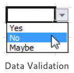
Data Validation lists are ideal not only where you need to make sure that people make the right entry but also for data entry generally as it is so easy to choose from a drop-down list. To create the validation list, select the cell or range of cells where you want the list to be displayed and then click the Data Validation control on the Data tab (look for Data Validation in the Data menu if you are using an older version of Excel)
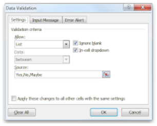
In the Settings tab, choose List from the Allow drop-down list and then type in a comma-separated list of your valid entries into the Source box. In this case, the list items are Yes, No and Maybe. Click the OK button and you’re done. The list is available when you click on one of the cells where the validation has been applied and data entry into the cell is restricted to only those items in the list.
Click the Error Alert tab if you want to change the standard “the value you entered is not valid” error message for invalid entries. You may prefer something a little more personal.
Using a range of cells to provide the source
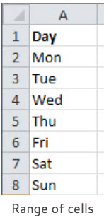
A range of cells is preferable for your data validation where you either have a long list or you want to be able to change the list regularly.
You can set the Source data validation as either a horizontal or vertical range of cells or an entire column or row. Either type in the range reference or (far easier) select the range or click the column letter or row number.
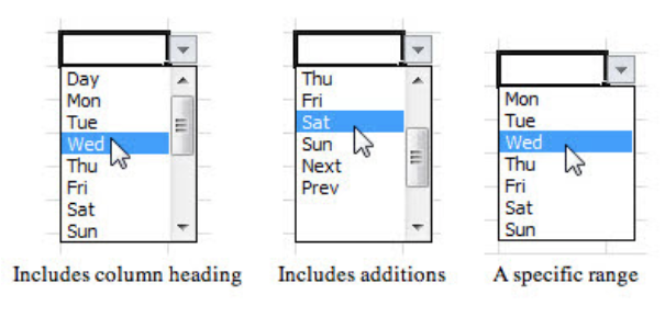
When you click the column letter remember that any heading at the top of your list on the worksheet will be included as the first item in your validation list. But if you add to the list on the worksheet then these additional items will automatically appear in the validation list. So there are advantages and disadvantages to selecting the whole column.
If you specify a range of cells then then you don’t have the headings issue to deal with but if you then add to the list on the worksheet then you will also have to remember to reset the Source data range to include your additions.
Displaying the drop-down list in alphabetical order
Dependant Data Validation lists
Sometimes you need the choice that you have made in one list to control the list shown in another cell; one of your validation lists is dependant on the other.
In the illustration there are two columns, the first column shows the class of date required, “Month” or “Day”. This is entered from a simple comma separated validation list which is typed in. The second column needs to show either a list of months if “Month” is entered in the corresponding cell in the first column or a list of days if “Day” is entered.
There are two ranges of cells in the worksheet named as Month and Day respectively which are going to be the alternative source ranges for the second column (see the next section if you are not sure how to Name a range) When you set the source data range for the second column enter the following formula: =INDIRECT(A2)
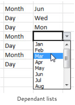
Where A2 is the first cell in the first column where you have your “Day” or “Month” entry. Of course, you should change this cell reference to suit your own worksheet. The INDIRECT function is well named as it makes the reference indirect, i.e. not A2 but the range reference entered in A2. In other words, if it’s “Day” then show the Day list, if it’s “Month” then show the Month list. You’re not restricted to just having a choice between two alternative lists, with this method you can have the choice of as many different lists as you like.
If this does not seem to work for you then try checking the following points:
- Did you select the area for the dependant range before applying the Data Validation? In the example above it would have been the second column. It’s very easy to apply validation to a single cell when you intended to set it for a range.
- Check the spelling of the range names (in this case “Day” and “Month”) in the first list. They must be spelled correctly and you have to remember them as you type them in as comma separated values.
- Did you remember to name the ranges?
Naming a Range
If you’re not sure how to name a range of cells then I would recommend using the Name Box, which is that area on the extreme left-hand side of the formula bar where you normally see your active cell reference. It’s not the only way of naming a range but most people find it to be the easiest way.
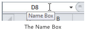

Type in the name (in this example it is “Months”) and then press the ENTER key to register the name correctly. Please don’t click out of the box after typing the name, press ENTER. Sorry for being boring but that’s where it’s so easy to go wrong. Click the drop-down arrow to check that the name is available.
Combo box and List box controls
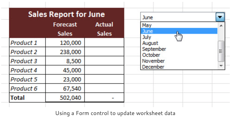
In the above example, there is a combo box control containing a list of months. When a month is selected from the list the heading in the worksheet report is updated (“Sales Report for …”) and the relevant monthly numbers are extracted from another worksheet where the full twelve month’s Forecast Sales figures are entered.
All this is done by using Excel formulas but you don’t need to know anything about the formulas to use the worksheet. You just choose a month from the drop down list. Combo box and List box controls are quite easy to do, the hard bit is doing all the formulas.
Form controls
Finding the Form controls
This is the first job. Form controls are not openly available, you need to display the Developer tab on your Excel ribbon. Click the File tab and then click Options. Click Customize Ribbon and then click the Developer check box in the Main Tabs list on the right-hand side. Click OK. Form controls are in the Insert control on the Controls group of the Developer tab.
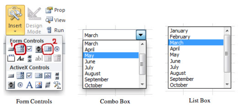
Click the Insert control, the Form Controls are the top group. The Combo Box (1) control is the second one in from the left. The List box (2) control is second in from the right. Both controls behave the same; the Combo box is a drop-down list, the List box is an open list.
Creating the Combo Box
You need to go through a few steps to get the Combo box working. Firstly, create some cell ranges where you are going to store the data that you want to have displayed in the drop-down list and a cell to link the Combo box to. When you format your Combo box these ranges are going to be your Input range and your Cell link.
Personally, I would always put these data ranges on a separate worksheet so that I can then hide it. In the example I shall be using Named Ranges, as they are so easy to work with, rather than normal cell references but this is just personal preference. Use Named Ranges or the standard A1-style cell references as you prefer, they both work fine.
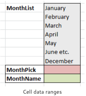
In the illustration, I have a list of my twelve months (shortened for clarity) these are the grey cells and are named MonthList. The pink cell is going to be the cell link and is named MonthPick and the green cell is MonthName, where I am going to enter a formula which will calculate the current month. Now it’s time to create the Combo box, there’s three steps:
- Draw and format the Combo box
- Set the Input Range and Cell Link
- Test the Combo box and the enter the formulas
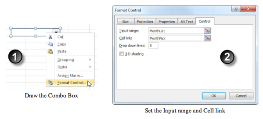
- Draw the Combo box. Click the Combo box control and then drag to draw a horizontal rectangular shape. You can resize it later if it’s not quite right. Right-click the control to display its shortcut menu. Try to right-click when your mouse pointer is pointing to the middle of the control as there are different shortcut menus available, you want the one that contains Format Control.
- Format the Combo box. In the Format Control dialog enter the Input Range (in this example MonthList) and the Cell link (MonthPick) Click OK.
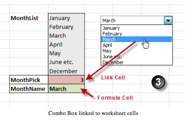
- Test the Combo box. Click a worksheet cell to take the focus away from the Combo box. It’s now active. Click the drop-down arrow and choose an item from the list. You should see that a value is returned into your link cell. It’s an index value, it’s not the text from the list. If you choose “March” from the list then the index is the value of 3 because it’s the third item in the list.
That’s the Combo box control completed and now it’s time to enter our formulas in the worksheet to make everything happen.
Entering the formulas
When you choose a month from the list you want to trigger the following processes in your formulas:
- Update the month name definition. This formula goes in the cell named MonthName so that we can use the name in our formulas wherever we need the selected month declared.
- Update the report heading with the name of the month.
- Update the report by showing the relevant data for the selected month.
1. Formula in the MonthName cell
Use the index value MonthPick to return the relevant item from the MonthList list using Excel’s INDEX function. The formula is:
=INDEX(MonthList,MonthPick)
2. Update the report heading with the name of the month
The named range MonthName updates to show the currently selected month so we concatenate it’s value with the static text “Sales Report for …”. This formula is entered on the worksheet where we have our report. The formula is:
=”Sales Report for “&MonthName
3. Update the Sales Forecast figures to show the currently selected month
There’s various ways of doing this but the most obvious way is to use the index value MonthPick in a Lookup formula to return the current month’s figures from the range containing all the year’s Sales Forecast figures.
