Excel - Mouse Training London Ltd

Excel AutoSum Revisited

You just can’t get away from AutoSum. If I had a pound for every time I’ve clicked AutoSum to add up a column of numbers I would probably be sitting on a tropical island somewhere still clicking it to add up all my vast wealth. It’s one of the first things you learn about in Excel and, of course, everybody knows it inside out.

Column and Row Totals

Here’s a really easy way of calculating column and row totals without having to do all that infernal copying. The first job is to select all the cells containing your numbers and extend the selection to the empty cells where you want the totals.

Then you click AutoSum and you’re done! It really is that easy. If you only want the column totals then just select the cells with the numbers and the totals are returned into the row below.

Here’s all the column and row totals done in two simple steps. And they are done perfectly as the range references in the SUMs are implied by the selection. They hardly need to be checked.

If you prefer to do the whole thing with your keyboard then hold down the SHIFT key and extend the cell selection by pressing the arrow keys. Then use the shortcut key combination ALT= to generate the SUM formulas.

Grand Totals

But it’s not just one table is it, you’ve got loads of them and some serious number crunching to do. You can extend the select-and-click-AutoSum method to do grand totals as well. But, be careful, this method only really works if every line item in your worksheet is drawn into a subtotal.

Firstly, calculate all of your individual subtotals and then make a selection of all of the cells containing your numbers and the cells containing your subtotals.

Now, click AutoSum and all the cells containing your subtotal SUMs are detected and the Grand Total is calculated correctly without any risk of double-counting.

Here’s the resulting formulas displayed in the cells and you clearly see the formulas containing the original range references for the subtotal SUMs.

All the grand total SUMs generated by AutoSum are Unions, showing each subtotal reference separated by commas. Number-crunching never has been much fun but this certainly better than having to construct Grand Totals from plus signs and cell references.

Our SUM formulas usually contain Range References, using a colon separator. For example, C3:C5 means “from C3 to C5”. Union references use commas. For example, C12, C16 means C12 and C16.

Checking your Formulas

As some of us know from bitter experience it is very embarrassing when a simple mistake in your formulas messes up all your careful calculations. So, it’s always a good policy to check that you’ve got your formulas right but it’s a bit painful to view them individually in the formula bar.

You can display the formulas directly in the cells by clicking the Show Formulas control. It’s in the Formula Auditing group of the Formulas tab. Click once to show the formulas and click again to show the results.

If you have a really old version of Excel then you have to search in the Tools, Options dialog for this option which is not much fun and I recommend that you use the shortcut key combination CTRL ` (that’s usually the key under the ESC key on the top right of your keyboard) Press the keys once to display the formulas and again to show the returned results.

Related Courses

Microsoft Excel Intermediate – Link

Microsoft Excel Advanced – Link

Excel Top Ten Shortcut Keys

Ask ten people what their favourite Excel shortcut keys are and you’ll get ten different answers. In no particular order, here’s my personal choice of the ones that I can’t do without. I’m not going to list ALL the Excel shortcut keys here because there are hundreds of them.

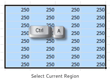
Ctrl+A Select the Current Region

Click a cell, press Ctrl+A and Excel expands your selection to select the Current Region. Press Ctrl+A again and the entire worksheet is selected.

The Current Region is defined as the current area of continuous data bounded by blank cells. In older versions of Excel you may have to press the key combination Ctrl+* to achieve the same effect (Ctrl+SHIFT+* if you don’t have a dedicated *key)

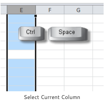
Ctrl+Spacebar Select the Current Column

What, pick up my mouse and click the column letter. No way! Ctrl+Spacebar selects your current column and then to extend the selection to the left or right you hold down the SHIFT key and use the Left or Right arrow key

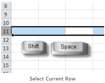
SHIFT+Spacebar Select the Current Row

Well, I did say that it’s a personal choice. Lazy-bones here selects the current row with SHIFT+Spacebar. Then keep the SHIFT key held down and press the Up or Down arrow keys to extend the selection up or down.

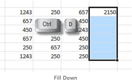
Ctrl+D and Ctrl+R Fill Down and Fill Right

Fill formulas or data down the column by selecting down with the SHIFT and Down arrow key. Then Ctrl+D fills down the selection. Ctrl+R to fill across to the right.

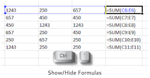
Ctrl+` Show/Hide Formulas

You can’t check that you’ve got your formulas entered correctly if you can’t see them.

Switch between displaying the returned results of your formulas and the actual formula itself by pressing Ctrl+` (that’s usually the key under the ESC key in the top left hand corner of the keyboard)

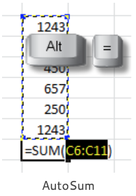
ALT+= AutoSum

Instead of clicking the AutoSum control every five minutes ALT+= enters a sum formula into the active cell. But it only does SUM and does not give you a choice of other functions.

See my article AutoSum Revisited for a few ideas on getting the best out of AutoSum.

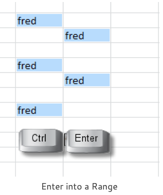
Ctrl+ENTER Range Entry

Pressing the ENTER key makes an entry into your current active cell. Ctrl+ENTER makes an entry into every single cell in your current selection. Make the selection, type in your entry and then press Ctrl+ENTER.

Constants (text or numbers) and formulas can be entered into a range in a single step. Formulas give you a relative reference for each cell, so if you get the first one right then all the others will adjust accordingly.

To enter data into a discontinuous range, make a multiple selection first. Select a cell or a range of cells then hold down the Ctrl key as you add to your selection by clicking on other cells or ranges.

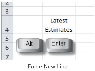
ALT+ENTER Insert New Line

Rather than wrapping the text in the cell whenever you want to force a new line press ALT+ENTER.

This is very handy for creating Excel source data for Tables or Pivot Tables where you maybe need to have multiple lines of descriptive text for a heading but retain the integrity of the single physical header row.

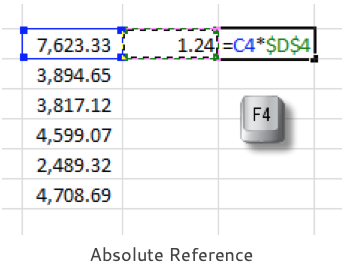
F4 Absolute Reference and Repeat

When you need Absolute References (dollar signs) in your formulas press F4. Succeeding presses of the F4 key return all the permutations of absolute and relative reference: $A$1, A$1, $A1, A1.

To make a single cell reference in your formula absolute, click somewhere on the reference then press F4. For a range reference or a series of references, drag across the references first before pressing F4.

F4 has a double life, when you are in Ready mode (i.e. not editing your formulas) F4means Repeat. Say you have the tedious job of going through a worksheet and deleting some of the rows, delete the first one as you usually do and then select the next row to be deleted and press F4 to repeat the row deletion.

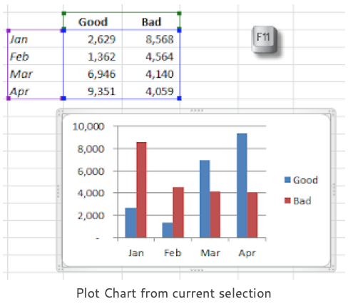
F11 Chart

Pressing F11 plots a default chart on a separate chart sheet based on your current cell selection. Press ALT+F11 for an embedded chart on the active sheet. Excel will automatically execute a current region selection if you start with a single cell selected in your chart data range. To plot discontinuous ranges, make a multiple selection using your Ctrl key before pressing F11.

Related Courses

Microsoft Excel Intermediate – Link

Microsoft Excel Advanced – Link

Excel Sort by Last Name

Excel Sorting By Last Name

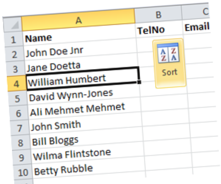
You have a list of names in your Excel spreadsheet with both the first and the last names in the same cell and you want to sort your list alphabetically by the last name. Not too much to ask, is it?

The bad news is Excel sorts on the entire entry in the cell reading from the left hand side and you can not specify any particular element of your text to provide the sort order. I know that’s what you want but you just can’t have it. Sorry.

Isolating the Last Names

The only way to do this is to get the last names into a separate column and then base your sort on that column and not on the existing names. Make sure that the sorting column is right next to one of the existing columns in your worksheet so that Excel captures it as part of your list. You can always hide your sorting column.

There are several methods of isolating the last names. In this article we shall be discussing Flash Fill, Text to Columns, Find and Replace and Formulas. To make your life easy, try to make your text as regular as possible as most of these processes are about finding a space in the middle of a bit of text. Any double-barrelled names like Ann Marie, Jean Paul or Wynn Jones will be much easier to process if you substitute the space with a dash, like this: Ann-Marie, Jean-Paul or Wynn-Jones.

Using Flash Fill

What could be easier, type in a few suggestions (I did Doe and Doetta) and then shoot over to the Data tab and click the Flash Fill control which you should be able to find in the Data Tools group. To be fussy, I could say that I really wanted to have Wynn-Jones instead of Wynn so I should have included one as an example but it’s only for sorting so I’m happy.

What’s your problem? You’re looking at your Data tab and you don’t have a Flash Fill control? That’s because it’s new with Excel 2013.

That’s the problem with this method; you need the software. You either have to buy a new copy of Excel or check out the rental version on Office 365.

Flash Fill is far and away the best method for this exercise and I would throughly recommend it as the program is so good at picking out patterns from your examples. The only drawback is that you would have to repeat the exercise whenever you added new names to the list. It’s worth buying a new copy of Excel just for Flash Fill.

Using Text to Columns

Text to Columns is where you can use the space between the first and last names as a “delimiter” and have Excel generate two columns of data; one with the first names and the other with the last names. You delete the first names column and keep the last names as your sort column. There will be issues with titles, middle names and initials etc.

This is Step 1 of the Text to Columns Wizard and here you just need to specify that you are processing Delimited data and then click the Next button to move on to Step 2.

Step 2 is where you specify the Delimiter; clear the Tab check box and click the check box for Space then examine the Data preview. As you can see, it’s not perfect as every space character has been used as a separator but it has done the bulk of the work so click the Finish button.

Here’s the resulting text, it’s been chopped-up (or parsed) into separate fragments based on wherever a space character was found in the original text. There’s still a bit of work to do as you need to delete the unwanted columns. It’s always a good idea to insert a few extra blank columns into your worksheet before using Text to Columns as this will avoid your accidentally over-writing any existing data.

Using Find and Replace

Again, this is all about using the spaces as separators and employs two passes of Find and Replace in combination with wildcards. This is definitely one for all the Find and Replace fans, I am constantly amazed at how creative and ingenious some people can be with Find and Replace.

Click the column letter at the top of one of your columns where you have the names and then replace every space with an arbitrary character, in this case an @ sign. You can use any character you like, just make sure that it’s a character that would not be found in any of the names. Type a space into the Find what box and an @ sign into the Replace with box then click Replace All. Now all the names look something like this: Bill@Bloggs, John@Smith etc.

The next job is to strip out all the text up and including the last @ sign by replacing it with nothing which will then leave the last text element which is, of course, the last name. Type the following expression into the Find what box, ?*@ and leave the Replace with box empty. Click the Replace All button and you are left with the last names.

The wildcard characters used here are the question mark, ? which means “Find any type of character” and the asterisk,* which means “Find everything”. Therefore ?*@ means “Find everything leading up to and including the last @ sign”.

Using Formulas

And then there are the Excel fans who would not dream of using Find and Replace because, for them, everything is done with formulas and functions for they can not be parted from their commas and brackets. The formula solution uses Text functions and is quite complex but it is constructed in stages; use the FIND or SEARCH function to read the text from the left hand side to find the position of the first space character. Then use the RIGHT function to extract the text after the space.

This is the first step, locating the first space in the first cell:

=FIND(” “,B2)

This formula gives the result of 5, the first space is located at character index 5, after the first four characters, “John”. The FIND function is case-sensitive which does not matter if you are finding a space but it could be an issue for some other characters, in which case you should use the SEARCH function which is not case-sensitive.

The next job is to extract the text from the right hand side up to, but not including, the space character which has now been located. Of course, the names are of varying length so you need to calculate how many characters in from the right hand side for which you need the LEN function. So the LEN of the cell minus the FIND value gives the number of characters required.

Here’s the finished formula:

=RIGHT(B2,LEN(B2)-FIND(” “,B2))

Be careful with the commas and the brackets if you are hand typing or click the Insert Function (fx) button and let Excel do them for you.

The final job is to copy the formula down the column and extract all the last names.

You can leave the formulas in the cells as it will not affect the sorting and it will make any additional records much easier to process as you can just copy the existing formulas.

A final thought, why didn’t we have two columns in the first place? Then we wouldn’t have to have Excel sort by last name. The moral of the story is to store things like first names and last names in separate columns.

Related Courses

Microsoft Excel Intermediate – Link

Microsoft Excel Advanced – Link

Excel Dollar Signs

Excel Absolute References, the Dollar sign $ and the F4 key

Excel Dollar Signs or, to be correct, Absolute References are one of those things that you really need to know about if you want to be successful with your Excel formulas. And it’s good idea to know about the F4 shortcut key.

Way back in the last century we always used to say that if you didn’t know your function keys then you weren’t being serious. Thankfully, those days have passed but you still need to know the F4 key for working with Excel formulas. The F4 key will repeat the last command or keystroke when you’re working in Word, Excel or PowerPoint. However, it’s primary use in Excel is for inserting the dollar signs ($) for Absolute cell references in your Excel formulas.

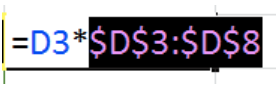
You may have seen cell references in formulas surrounded by ‘$’ signs, for example $D$3:$D$10, and wondered what’s that all about? The ‘$’ before the column or row reference fixes the reference so that it does not change when it’s copied. You either have to type in the $ signs or press the F4 key. Be careful with the F4 key on your laptop, if it does not seem to work properly then press Fn and F4 together. Press CMD+T if you’re working with Excel for Mac.

Using Absolute References in Formulas

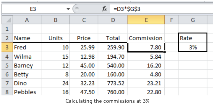
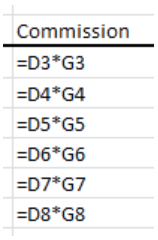
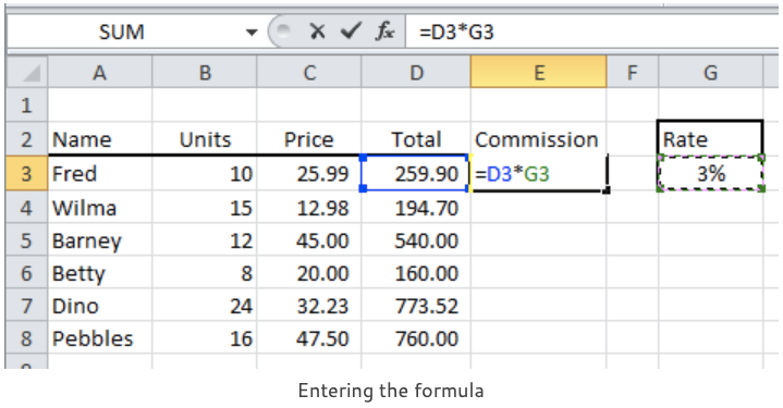
For example, looking at the table above we have a Commission Rate of 3% in cell G3. In column E we want to calculate the commission as Total x Rate @ 3%. We could simply enter the formula as =D3*3% and copy it down column E, but then that gives us two major problems to deal with:

We can’t easily see what the commission rate is without looking in the formula bar. We could include it in the column heading as “Commission @ 3%”, but that makes the heading too wide and if I should change the rate then I will have to remember to go back and change the heading as well.
If I do change the rate then I need to change the formula and copy it down the column again. Doing this once would be acceptable but not if I need to do it regularly and what if other formulas are using the commission rate? It would be so much easier just to have the commission rate in a single cell.

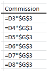
In the formula for the commission calculation, the commission rate of 3% is entered into cell G3 and then the G3 reference is used in our formulas like this, =D3*$G$3. The reference is absolute, meaning that it never changes wherever the formula is copied.

Let’s look at what happens if we don’t use an absolute reference. If we entered in cell E3 the formula =D3*G3 we would get the correct answer. But when we copy that formula down the rest of column E Excel updates the cell references in the formula to increase by one row as we go down. You can see this to the left where the references to D3 and G3 change to D4 and G4 etc.

These standard cell references are known as relative references. We want the D3 reference to change but we want the G3 reference to be fixed.

To keep the commission rate reference on cell G3 we enter the formula like this, =D3*$G$3. Then when we copy the formula down the column the column D references change but the reference to cell G3 does not.

Strictly speaking, we only needed to fix the reference to row 3 as the G column reference would not have changed but it’s usually easier just to fix the entire cell reference and have done with it. The difficult bit is to realise that you needed an absolute reference in the first place.

Other ways to use Absolute References

Make a whole range of cells an absolute reference: $D$1:$F$1
Make only the column absolute: $D3
Make only the row absolute: D$3

To help you see how your formulas are behaving it’s quite a good idea if you can actually see them instead of the results of the formula. To display your formulas in the worksheet, click the Show Formulas control on the Formula Auditing group of the Formulas tab.

F4 Shortcut for entering Absolute References

The F4 key instantly enters the ‘$’ signs for you. You can do it while you’re entering your formula or you can go back and edit the original formula.
In the example below we have started to enter a formula into cell E3. We have just selected cell G3, as you can see by the marquee (“marching ants”) around the cell.

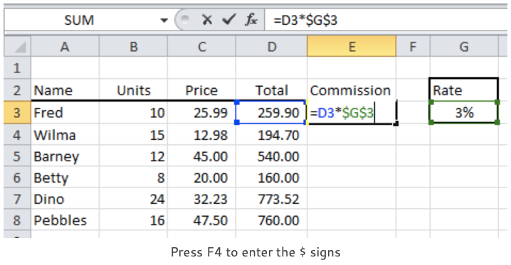
At this point, before pressing ENTER or clicking the tick to finish the formula, we can press the F4 key and Excel places the ‘$’ signs around the G3 reference. Or you can go back to a cell at any time. Press the F2 key to edit the formula if you are feeling old-fashioned, or just double-click the cell. Click anywhere in the cell reference and press F4 to insert the $ signs.

If you want to fix a range reference you have to highlight the cell range in the formula before pressing F4. If you keep pressing F4 Excel iterates through all the permutations of absolute and relative reference:

With the first press of F4 you get $G$3. Column and row absolute.
With the second press of F4 you get G$3. Column relative and row absolute.
With the third press of F4 you get $G3. Column absolute and row relative.
With the fourth press of F4 you get G3. Column and row relative.

Mixed Relative and Absolute references

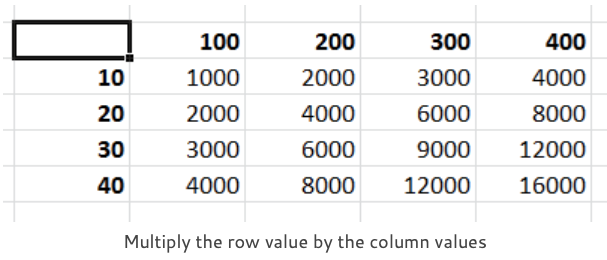
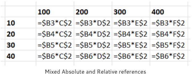
Whilst it usually easier to fix the entire reference there are times when you must have a mixed reference, where only the row or the column is fixed, in order to make your formulas work. In the worksheet example below we are multiplying all the hundreds values in the top row against all the tens values in the first column of the table. The first formula multiplies the 10 by the 100, =B3*C2.

As the formula is copied across and down we need the row reference for the hundreds values to be fixed and the column reference for the column reference for the tens values to be fixed. But the rest of the formula must be relative so that it works correctly when it is copied.

Usually I try to work out this type of formula logically before I start. And usually it goes wrong so I just resort to experimentation until I get it right. It only takes me an hour or so. Best of luck with your Excel Dollar Signs!

Related Courses

Microsoft Excel Intermediate – Link

Microsoft Excel Advanced – Link

Microsoft Excel Flash Fill

Excel – Flash Fill

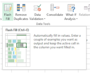
Sometimes, half the problem is getting data into Excel so that you can work on it. You run a query on a database and get a mishmash of poorly formatted data. Hundreds of rows full of data you don’t want mixed with the few odd bits that you do. Been there? This is where you need Excel 2013’s Flash Fill to come to your rescue.

To make sense of your data, type in a few row’s as an example of what you need and then click Flash Fill to do the rest of the work for you. Excel applies the lessons learnt from your examples to the rest of the data, with all the columns below filling with the correctly formatted data. No complicated formulas and no macros required. And no retyping!

You can extract simple patterns from your data, for example extract the first name from a full name or you can extract multiple patterns. For example, you can get the date, the business name and the amount from a credit card statement. All by typing a couple of examples for Excel to use as a template.

The Microsoft Excel Flash Fill control is on the Home tab of the ribbon in the Fill group. It is also found in the Data Tools group on the Data tab. And, of course, you can add it to your Quick Access Toolbar if you find yourself using it frequently.

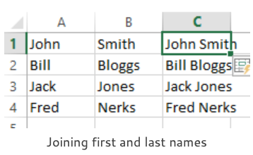
Flash Fill Example

Here’s a simple exercise; joining first and last names together in the same cell. Type the example “John Smith” into column C and then click Flash Fill to do the rest.

That’s an easy one. If you know Excel formulas you could do that as
=A1&B1 or =CONCATENATE(A1, B1)

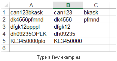
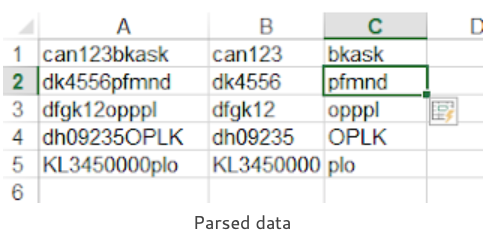
Let’s try the Microsoft Excel Flash Fill challenge, a really hard one. In this exercise we need to parse the data in the first column so that a series of numbers appearing after a series of letters is identified and the text after the series of numbers is extracted.

I am getting a headache just thinking about how I would do this one with a formula…

Begone with your complicated formulas and Text-to-Columns routines. Type-in a couple of examples and let Flash Fill take over. The results are seriously impressive.

Try doing that with a formula. I’ve still got that headache.

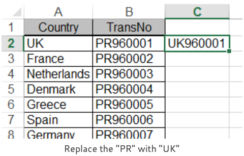
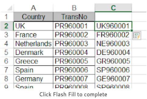
Let’s try one more; here we need to remove the two-letter prefix “PR” from the front of the entries in column B and replace it with the first

two letters of the country entered in column A. As capital letters.

Enter the first item in column C to set the pattern and then click Flash Fill to do the rest. Fantastic!

Well, I think that we could have done this one using the LEFT, RIGHT and UPPER functions to extract and convert the relevant data. Then concatenated the results to produce the new transaction code.

But the point is, we don’t have to do that sort of thing any more and I for one will not miss it at all. This is the kind of machine learning and artificial intelligence that we all appreciate.

Related Courses

View Excel Training Courses – Link

Switching Excel Columns to Rows

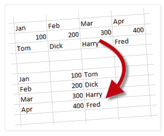
Switching Excel Columns to Rows. You should really call this Transposition if you want to impress. Excel data can be rearranged from columns to rows and vice versa. You can transpose as many rows or columns as you like all in one go. You need to decide whether you want to do the transposition just once or have the transposed data update to reflect any changes made to the original.

Static Transposition

Static transposition is where the data is rearranged just once and it’s really easy to do. However, dynamic transposition, where you have two sets of Excel data; one arranged in columns and the other in rows, is much more difficult and involves your entering an array formula.

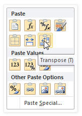
If you know how to Copy and Paste then you’ll find static transposition a breeze. The copy bit is as normal but there is a variation to the paste bit. Select the original range of cells and Copy them. Then click a blank cell that is away from the original range and Transpose; there is no need to select the entire range for the transposition, a single cell is all you need.

Finding the Transpose command depends on which version of Excel you are using. If you have a modern version of Excel with the fancy ribbons then you should be able to find Transpose in the Paste control on the Home tab or in the shortcut menu when you right-click.

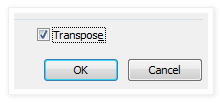
Should you have one of the good old fashioned versions with the drop-down menus then look for Paste Special which is found in the Edit menu. Failing that right-click after you have done your Copy and you may very well find Paste Special in the shortcut menu.

When the Paste Special dialog appears you need to find the Transpose check box, give it a click and then click the OK button. Sounds easy doesn’t it? But I often find myself staring at the screen muttering “now, where’s that Transpose thingy…”. Because it’s right down the bottom, where it always has been.

Dynamic Transposition

In the previous example we transposed our data and ended up with two independent ranges of cells, one of which you would probably want to delete. You might want to keep both ranges and have the transposed data change when changes were made to the original. This where you need to have a formula. The most painful method would be to go through each cell, enter an equals sign and click the corresponding cell in the original range. Very tedious indeed.

A much better method would be to create an array formula using the TRANSPOSE function. Array formulas are not easy to enter and most sensible people run screaming from the room at the mere mention of them. So don’t get annoyed if this formula takes a few goes to get right. Like most Excel formulas you have to persevere and suffer for a bit until you feel confident.

Entering an Array formula

Array formulas are entered into ranges of cells in one go. They are not entered into single cells and then copied which is what we are used to. You select the range, enter the text of the formula and finally, press CTRL+SHIFT+ENTER on your keyboard to enter your formula into the selected range.

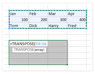
The first job is to count the number of rows and columns in the range that you wish to transpose. Then select a range of empty cells whose dimensions correspond to the inverse of the original range. For example, I want to transpose the range D4:G6, which is a range with 5 columns and 3 rows, so I select an range of 3 columns by 5 rows.

Now we enter the required formula. The formula is as follows “=TRANSPOSE(D4:G6)”. Then, holding down the CTRL and SHIFT keys, press ENTER or click the Enter box in the formula bar.

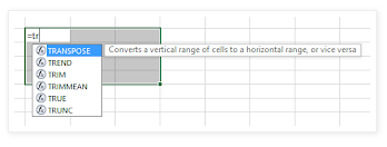
If you have a version of Excel that pops up the list of functions as you type then you can accept TRANSPOSE from the list by pressing the TAB key. Array formulas are identified in the formula bar enclosed in braces (the squiggly brackets) but you do not type in the braces when you enter the formula.

Working with Array formulas

You may not change part of an array formula. If you want to delete your formula, select the entire formula first before pressing the Delete key. To edit the formula there is no need to select the whole array first but don’t forget to press CTRL+SHIFT+ENTER to accept the edit.

The Excel shortcut key to select the current array is CTRL+/ (front slash). If you have a huge transposition just click one cell and then the short cut key will select the rest of it for you.

When you are counting the number of columns or rows in a large range it is all too easy to lose count and very frustrating when you have to start over again. “One, two, three, four… ” Such fun. Use the Excel functions ROWS or COLUMNS to calculate the dimensions of large ranges rather than count them. For example, the formula =ROWS(A1:D50) returns the value of 50.

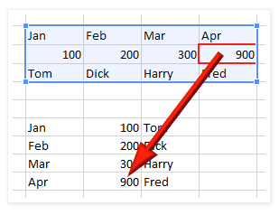
Transposition formulas are not the easiest of formulas to get right but, like all formulas, once they are done they will look after themselves and update automatically.

Any changes made to the original range are immediately reflected in the transposition.

Related Courses

Microsoft Excel Intermediate – Link

Microsoft Excel Advanced – Link

Training Courses

If you’ve still got that “I just don’t know what I’m doing” feeling then you might like to arrange an Excel training course for yourself or with some of your colleagues. It’s really easy to book one of our courses and they’re great value for money. See our website for full details.

Switching Excel Columns to Rows by Mouse Training London

Excel AutoSum Revisited

Table of Contents

Excel AutoSum Revisited

Column and Row Totals

Grand Totals

Checking your Formulas

Related Courses

Excel Top Ten Shortcut Keys

Table of Contents

Excel Top Ten Shortcut Keys

Ctrl+A Select the Current Region

Ctrl+Spacebar Select the Current Column

SHIFT+Spacebar Select the Current Row

Ctrl+D and Ctrl+R Fill Down and Fill Right

Ctrl+` Show/Hide Formulas

ALT+= AutoSum

Ctrl+ENTER Range Entry

ALT+ENTER Insert New Line

F4 Absolute Reference and Repeat

F11 Chart

Related Courses

Excel Sort by Last Name

Table of Contents

Excel Sorting By Last Name

Isolating the Last Names

Using Flash Fill

Using Text to Columns

Using Find and Replace

Using Formulas

Related Courses

Excel Dollar Signs

Table of Contents

Excel Absolute References, the Dollar sign $ and the F4 key

Using Absolute References in Formulas

Other ways to use Absolute References

F4 Shortcut for entering Absolute References

Mixed Relative and Absolute references

Related Courses

Microsoft Excel Flash Fill

Table of Contents

Excel – Flash Fill

Flash Fill Example

Related Courses

Switching Excel Columns to Rows

Table of Contents

Static Transposition

Dynamic Transposition

Entering an Array formula

Working with Array formulas

Related Courses

Training Courses