Office 365 Groups

Microsoft Office 365 Groups

Table of Contents

office 365 groups

What are Office 365 Groups?

Microsoft Office 365 Groups lets you to collaborate with your teammates when writing documents, creating spreadsheets, working on project plans, scheduling meetings and sending email. Office 365 release 2019 is a new service available to 365 and 2019 Outlook users.

Groups lets you choose a set of people that you wish to collaborate with and also set up a collection of resources for them to share. For example; a shared Outlook inbox, a shared calendar or a document library for collaborating on files.

You don’t have to manually assign permissions to all these resources because you automatically give the required permissions when you add members to the group. Any member of the group can use the tools that your group provides. Groups are the new and improved method for what we used to do using distribution lists or shared mailboxes.

Office 365 Groups can be created from:

  • Outlook on the web
  • Outlook Mobile
  • SharePoint
  • Planner
  • Teams

Which tool you choose to start from depends on what kind of group you’re working with. For example, most will tend to start from Outlook when creating a Group organised around email and calendar. If the Group is for company wide communication you would tend to start with Yammer. For chat-based collaboration start your Group from Microsoft Teams.

Creating Groups

When creating a group where you can collaborate with your teammates you need to decide if you want it to be a private group or a public group. Content in a public group can be seen by anybody in your organisation and anybody in your organisation is able to join the group. Whereas content in a private group can only be seen by the members of the group and people who want to join a private group have to be approved by a group owner.

Neither public groups nor private groups can be seen or accessed by people outside of your organisation unless those people have been specifically invited as guests.

Adding guests to Office 365 Groups

Guest access 

Office 365 Groups lets you and your team collaborate with people from outside your organisation by granting them access to group conversations, files, calendar invitations and the group notebook. Access can be granted to a guest—for example, a partner, vendor, supplier, or consultant—by any group owner.

How it works?

People using Office 365 Groups can use Outlook on the web or Outlook for Windows to add and manage guests in their Office 365 groups. Guests can have any email address, and their email account can be a work, personal, or school account.

Note: Guest access is set up by the IT administrator.

  1. A group owner adds a guest to the group or a guest is nominated by a group member. The group owner approves the nominees.
  2. The group owner is informed of which content and resources the guest can access within the group. A combination of text and icons gives all group members a clear indication of guest participation.
  3. The guest receives a welcome email and can participate in group conversations, receive and respond to calendar invitations, and access the group files.
  4. Guests can leave the group at any time via a link in the footer of all group email messages and calendar invitations.

Admins can manage guests and their access to Office 365 group resources using PowerShell. See Manage guest access in Office 365 Groups for instructions.
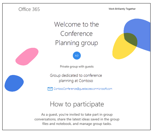
 

When a guest is invited to join a group, they receive a welcome email message that includes a little information about the group and what they can expect now that they’re a member. The message also includes a set of links to help them get started and connect to group resources.
OutlookGroups

The guest member’s interactions all occur through their email inbox. They can’t access the group site but can receive calendar invitations, participate in email conversations and, if the admin has turned on the setting, they can open shared files using a link or attachment.

All group email messages and calendar invitations the guest receives will include a reminder to use Reply all in responses to the group, along with links to view group files and leave the group.
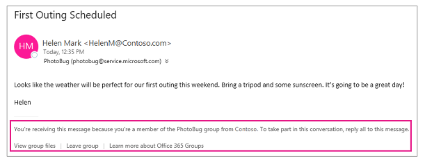
FirstOutingScheduled

The following table summarises what guests can and can’t do.
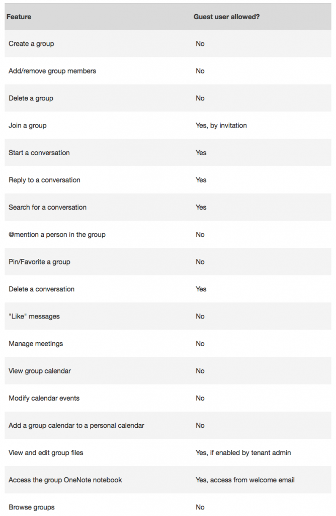
GuestCanAndCantDo

Excel- Automatically change the Pivot Table source data range

Excel Automatically change Pivot Table source data range

Table of Contents

pivot table refresh

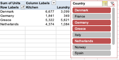
Excel- Automatically change the Pivot Table source data range. When you change the source data of a Pivot Table you need to click Refresh to reflect these changes. But if you add any new rows to the end or columns to the sides of the list, refreshing the data does not detect these additions to the original source data range. The best way to get round this problem is to convert your original range to an Excel Table and then use the table reference as the source data for your Pivot Table. The table reference automatically expands or contracts to fit the range.

Change data source

Pivot Table source data range

If you want to use the original range as your data source then you will have to update the definition of the Data Source by clicking the Change Data Source control on the Options tab of PivotTable Tools. And you will have to repeat this process every time you add any new rows to your list. This article shows you how to automate the process of redefining the source data range using a macro.

Changing the Data Source range automatically

We saw in an earlier article, Make Pivot Tables refresh automatically how to refresh a Pivot Table automatically using the Worksheet_Activate event macro.

You can change the Worksheet_Activate macro so that in addition to refreshing the Pivot Table it also updates the definition of the Data Source. Thus the Pivot Table responds to any additions or deletions made to the original data range. Copy and paste the section below into your Worksheet_Activate macro:

Private Sub Worksheet_Activate()

Dim PTRange As Range

‘Reset the data source and refresh.

Set PTRange = Sheets(“Sheet1“).Range(“A1“).CurrentRegion

ActiveSheet.PivotTables(“PivotTable2)”).ChangePivotCache _
ActiveWorkbook.PivotCaches.Create(SourceType:=xlDatabase, _
SourceData:=PTRange)

ActiveSheet.PivotTables(“PivotTable2“).PivotCache.Refresh

End Sub

You need to be a wee bit careful with the macro above and check the following:

  • The example assumes that your Pivot Table source data range is on “Sheet1” of the workbook and is a range that starts with cell reference “A1”. Should this not be the case then you must change the following line as required:
    “Set PTRange = Sheets(“Sheet1“).Range(“A1“).CurrentRegion”
  • The example assumes that the name of your Pivot Table is “PivotTable2“. To find out the name of a specific Pivot Table, right-click one of its cells and choose Pivot Table Options from the short cut menu.

Visual confirmation

If you want to visually confirm that your Pivot Table has been refreshed you can place an unobtrusive message down the bottom of the Excel window on the Status Bar. Add the following line to your Worksheet_Activate macro and clear the message away when you activate a different sheet using the Worksheet_Deactivate event.

Private Sub Worksheet_Activate()

‘The updating and refreshing macro goes here……see above

‘Show the message.
Application.StatusBar = “Pivot Tables updated at “& Time

End Sub


Private Sub Worksheet_Deactivate()

‘Clear message.
Application.StatusBar = False

End Sub

status bar

Excel’s Status Bar is visible at the bottom of the Excel window and your messages are always shown on the left hand side. If you don’t want the time stamp shown in your message then leave out the “& Time” part of the message.

I hope you managed to follow the “Excel- Automatically change the Pivot Table source data range” article. It looks complicated but it’s only really copying and pasting bits of VBA code.

Related Courses

Microsoft Excel Intermediate – Link

Microsoft Excel Advanced – Link

Excel – Make Pivot Tables Refresh Automatically

Excel Make Pivot Tables Refresh Automatically

Table of Contents

pivot table refresh

Excel – Make Pivot Tables Refresh Automatically. Excel Pivot Tables do not automatically update when their source data is changed. Unlike formulas they have to be refreshed. That’s no problem if you can remember to do it, but it’s all too easy to forget.

To make your Pivot Tables refresh automatically you need a Macro to do the refreshing and an Event to trigger the macro. You record a macro of your refreshing the Pivot Table and then you copy the recorded code and paste it into one of the worksheet’s events. This seems quite an involved process the first time you do it. But it gets easier every time you repeat it as it is just copying and pasting from one workspace to another.

Excel Refresh Pivot Table

Recording the Macro

Firstly, make the recording. Select a cell in your Pivot Table and then click the Record Macro control in the Macros group at the extreme right of the View tab.

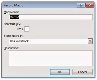
Make sure that the Store macro in: setting is This Workbook and click the OK button. Now you have to record your refreshing the Pivot Table; just right-click the active cell and choose Refresh from the shortcut menu. The recording is now completed and you have to turn off the macro recorder by clicking the Stop Recording control in the Macros group on the View tab.

RecordingMacro

The next job is to find the recorded code and copy the instruction that refreshes your Pivot Table. Click the View Macros control in the Macros group on the View tab, select your recorded macro from the list and then click the Edit button on the right hand side. You will now see your recording displayed in the Visual Basic Editor, it should look something like this:

SubMacro
Copy the line of code that refreshes the table. It should be obvious which one you need-the line is highlighted in the illustration above. Do not copy anything else. Now, exit the Visual Basic Editor and return to Excel by clicking an Excel icon or by pressing ALT+F11.

Using an Event to trigger the Macro

RightClick

Next, you need to find the Events for the worksheet where your Pivot Table is located. Every Excel worksheet has a collection of event-driven macros which trigger automatically whenever a particular event occurs. For example, the Selection Change event is triggered whenever you click a cell on the worksheet. We are going to use the Activate event to make our Pivot Table refresh.

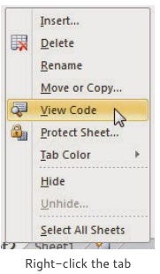
Right-click the worksheet tab and choose View Code from the shortcut menu. You are returned to the Visual Basic Editor once again but this time the screen looks blank. Don’t let that put you off, looking at the top of the active window you will see two drop-down lists.

The drop-down list on the left hand side is the Object list, the one on the right hand side is the Procedure list.
The Object List

Go to the Object list on the left and select the Worksheet object and then choose a suitable event from the Procedure list on the right.

Procedure List

All objects have default events and these usually appear in the window automatically, ignore them and scroll up the list to select the Activate event. Paste your recording into the event procedure so that it looks like this:

Event Window
The Activate event is triggered whenever you make that worksheet active, so in order to test that the procedure is working correctly you need to perform the event.

Return to the Excel workspace by clicking an Excel icon or by pressing ALT+F11, select another worksheet in the workbook and then return to the original worksheet where the Pivot Table is stored. This triggers the event and you will see that the tables are automatically refreshed. The best test is to change something in your source data and then see if your Pivot Table updates to reflect the change.

Using your Macro Again

Of course, you do not have to do the macro recording every time, all you need is the code for the Refresh method so you can type it in or paste it from a previous recording. But, be careful, each Pivot Table needs to be correctly referenced using its Name Property, this is the text value inside the brackets. In the example below the name of the Pivot Table is “PivotTable1”
 
ActiveSheet.PivotTables(“PivotTable1”).PivotCache.Refresh
 
To find out the name of a specific Pivot Table, right-click one of its cells and choose Pivot Table Options from the short cut menu.

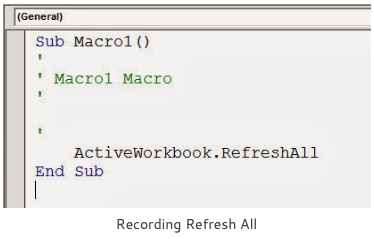
If you have several Pivot Tables that need to be refreshed then it is quite in order to list the various Pivot Tables one after the other in your macro but it is probably best if you recorded Refresh All in which case the initial recording would like the illustration on the right.

Saving your file

When your Excel workbook file contains macros remember to save the file in the Excel Macro-Enabled Workbook format.

Recording Refresh all

Make Excel Pivot Tables Refresh Automatically Summary

I hope you managed to follow all of this and you get a successful result. It’s only a macro recording and a copy and paste but well worth the effort as now you will never have to remember to refresh your Pivot Tables.

If you also need to automatically update the definition of the source data range before refreshing the data, see the article Excel- Automatically change the Pivot Table source data range.

Related Courses

Microsoft Excel Intermediate – Link

Microsoft Excel Advanced – Link