Category: Office 365
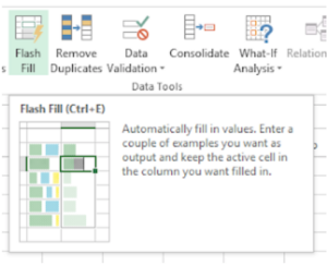
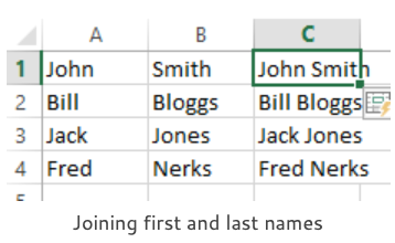
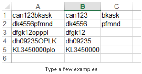
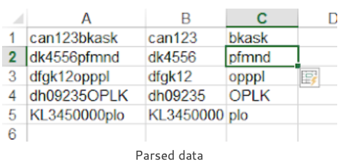
Microsoft Excel Flash Fill


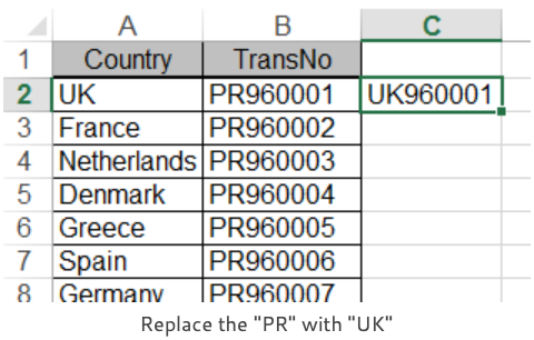
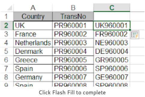
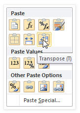
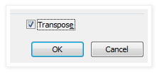
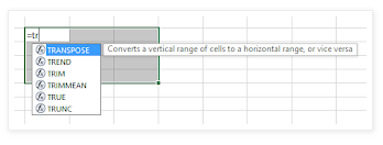
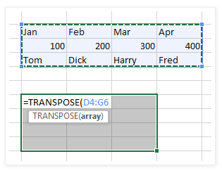
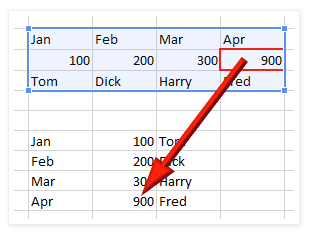
Switching Excel Columns to Rows


Office 365 Groups


