Microsoft Excel Flash Fill

Excel – Flash Fill

Sometimes, half the problem is getting data into Excel so that you can work on it. You run a query on a database and get a mishmash of poorly formatted data. Hundreds of rows full of data you don’t want mixed with the few odd bits that you do. Been there? This is where you need Excel 2013’s Flash Fill to come to your rescue.

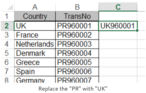
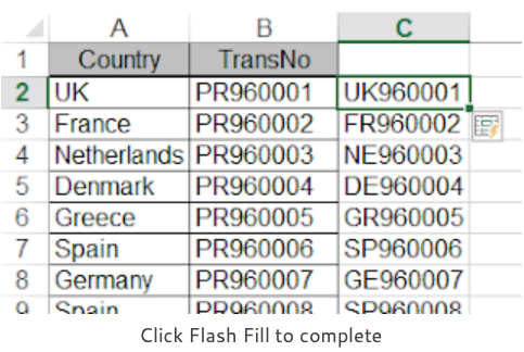
To make sense of your data, type in a few row’s as an example of what you need and then click Flash Fill to do the rest of the work for you. Excel applies the lessons learnt from your examples to the rest of the data, with all the columns below filling with the correctly formatted data. No complicated formulas and no macros required. And no retyping!

You can extract simple patterns from your data, for example extract the first name from a full name or you can extract multiple patterns. For example, you can get the date, the business name and the amount from a credit card statement. All by typing a couple of examples for Excel to use as a template.

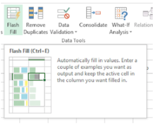
The Microsoft Excel Flash Fill control is on the Home tab of the ribbon in the Fill group. It is also found in the Data Tools group on the Data tab. And, of course, you can add it to your Quick Access Toolbar if you find yourself using it frequently.

Flash Fill Example

Here’s a simple exercise; joining first and last names together in the same cell. Type the example “John Smith” into column C and then click Flash Fill to do the rest.

That’s an easy one. If you know Excel formulas you could do that as
=A1&B1 or =CONCATENATE(A1, B1)

Let’s try the Microsoft Excel Flash Fill challenge, a really hard one. In this exercise we need to parse the data in the first column so that a series of numbers appearing after a series of letters is identified and the text after the series of numbers is extracted.

I am getting a headache just thinking about how I would do this one with a formula…

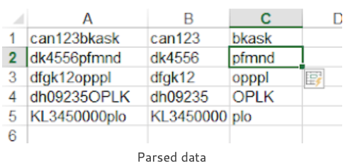
Begone with your complicated formulas and Text-to-Columns routines. Type-in a couple of examples and let Flash Fill take over. The results are seriously impressive.

Try doing that with a formula. I’ve still got that headache.

Let’s try one more; here we need to remove the two-letter prefix “PR” from the front of the entries in column B and replace it with the first

two letters of the country entered in column A. As capital letters.

Enter the first item in column C to set the pattern and then click Flash Fill to do the rest. Fantastic!

Well, I think that we could have done this one using the LEFT, RIGHT and UPPER functions to extract and convert the relevant data. Then concatenated the results to produce the new transaction code.

But the point is, we don’t have to do that sort of thing any more and I for one will not miss it at all. This is the kind of machine learning and artificial intelligence that we all appreciate.

Related Courses

View Excel Training Courses – Link